Non-normal data; PROC GLIMMIX

[AgReseach7]

Completed a feedlot Trial with 6 treatments (animal was exp. unit). We collected blood (twice) and analyzed multiple blood serum components (e.g., urea N, glucose, etc.).

Some of the continuous variables are not normally distributed.

Right now, I have the following SAS statement together, but need help on determining exactly what to use (run all of them and look at model with best fit?):

"Method = " laplace, quad or ?

"Dist = "  normal, gamma, invgauss, beta, or ?

"Link = " log or ?

"Adjust = " How do you know to use "Tukey" or "KR"?

I believe that ARH(1) will provide the best fit, but... do I need to also try CSH, AR(1), CS, ...?

There are too many possible combinations of the above factors, thus I'm sure I'd screw up somewhere.

Guidance on what to use would be much appreciated.

I attached an Excel spreadsheet of the data if needed (I highlighted the serum variables that I can't get "normal"; through data transformation, deleting any outliers that I can, etc...).

PROC GLIMMIX method=laplace;

CLASS TRT DAY ID;

MODEL GLUCOSE = TRT day trt*day/dist=negbin link=log;

Random day / subject = id(trt) type =ARH(1);

LSMEANS TRT day/PDIFF ADJUST=TUKEY;

LSmeans trt*day/slicediff=day adjust=tukey;

RUN;QUIT;

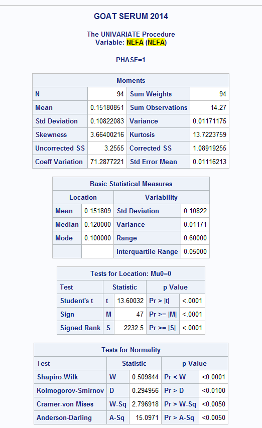
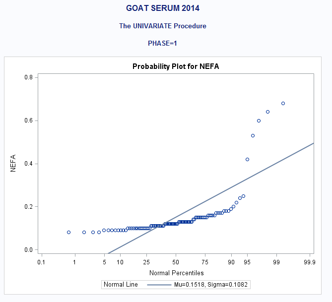
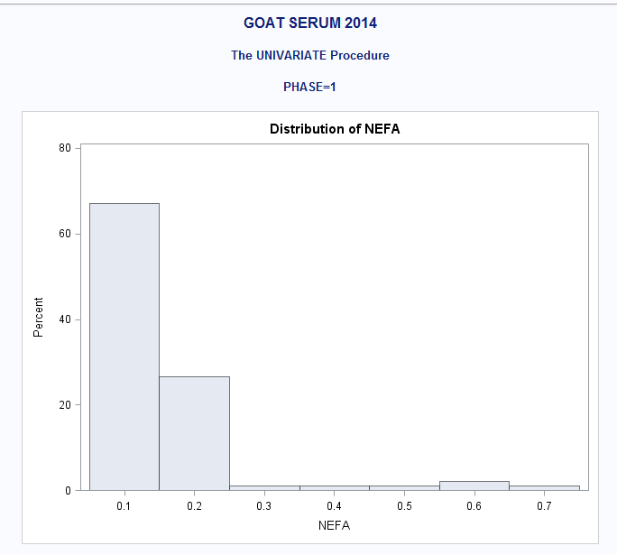
ALSO: PROC UNIV. of NEFA if it helps any

[SteveDenham · Accepted solution]

I would say some of the endpoints have a normal distribution of errors (remember that is the assumption, NOT that the endpoint itself is normally distributed)  The others are probably best fit with a lognormal distribution.

As far as the error structure, a lot depends on the spacing of the measurements in time. AR(1) and ARH(1) assume that the measurements are equally spaced in time.  CS and CSH assume that the correlation between close together time points is the same as more separated in time points.  However, you only have two time points (Day 0 and Day 26), so CSH and CS would make perfect sense.  Fit both, pick the one that yields the smaller corrected AIC value.  Try the following:

PROC GLIMMIX data=yourdata;

CLASS TRT DAY ID;

MODEL GLUCOSE = TRT day trt*day/dist=lognormal ddfm=kr2;

Random day /residual subject = id(trt) type =CSH;

LSMEANS TRT day/DIFF ADJUST=TUKEY;

LSmeans trt*day/slicediff=day adjust=tukey adjdfe=row; /* I really dislike Tukey's adjustment for repeated measures data.  You might look into adjust=simulate */

ODS OUTPUT lsmeans=lsmeans;

RUN;QUIT;

Now, to get lognormal estimates back onto the original scale you'll have to post-process the lsmeans dataset, and this is where some mathematical statistics enters the picture.  Simply exponentiating the estimate will give an estimate of the median value.  If you want to get an estimate of the expected value and of the standard error of the expected value, you'll need the following code:

data btlsmeans;

set lsmeans;

omega=exp(stderr*stderr);

btlsmean=exp(estimate)*sqrt(omega);

btvar=exp(2*estimate)*omega*(omega-1);

btsem=sqrt(btvar);

run;

Steve Denham

[AgReseach7]

Exactly what I needed. You saved me a couple of day and a few headaches.

MANY THANKS!

[AgReseach7]

In your post below, I am curious:

What is the difference in your editor statement vs. iLink function in an LSMeans statement?

[SteveDenham]

Because the variance is separable from the mean for the lognormal distribution, using the ILINK option with DIST=LOGNORMAL will return the same value on both the link transformed and original scales.  That is why you have to post-process.

Steve Denham

[AgReseach7]

how do I get beta (PROC GLIMMIX Beta distribution) back on original scale?