Proc nlin method

[GavinB]

I have a dataset with samples taken over time which looks as follows (took out one ID to show what it looks like):

Name	Time	X
1703187-01	0	2.07936
1703187-01	0	1.795714
1703187-01	30	21.24958
1703187-01	30	22.44529
1703187-01	60	34.25629
1703187-01	60	33.70213
1703187-01	90	44.95228
1703187-01	90	44.56428
1703187-01	120	54.86515
1703187-01	120	55.98709
1703187-01	150	66.58977
1703187-01	150	62.09209
1703187-01	180	80.25785
1703187-01	180	77.43605
1703187-01	240	88.45111
1703187-01	240	88.8228

I am using the Nlin method to solve the following equation: X=A + B * (1 - Exp(-km * :Time)) ^ c.

My code then looks like this: 

proc nlin data=IV plots=all maxiter=2000;
parms A=2.5 Km=0.004 B=65 C=1;
model X= A + B * (1 - exp(-Km * Time))**C;
output out=IV p=yhat r=resid u95=upper l95=lower
parms= A Km B C;
run;

This model will not fit properly if I try to run it on the dataset, however, if I change the Time values of my first time-point to for example 0.01 it does work. If I change them to 0.001 and run it again, it does not work anymore.

One of my collagues works in JMP and if he tries to fit the model on the original data it works perfectly, so I am really struggling to determine why it wont work in SAS, but more importantly, why it does fit when I change the first timepoint to something above 0. Does Nlin have issues with a 0 point?? 

[Rick_SAS]

You need to include DCt in the input data set.

[GavinB]

Hi Rick,

I see I made a mistake when posting this, X in the table above is the DCt. I have adjusted that now, but that was already okay in my input file SAS. So the issues still remains......

[Rick_SAS]

Please explain what you mean by "doesn't work." Is there an ERROR or WARNING in the SAS log?  If so, please append the log.

Is there non-convergence?  

We also need to know what version of SAS you are running. Submit

&put &=sysvlong;

and look in the log.

Lastly, since you did not post your data in the form of a DATA step, there could be an error in the way the data are read. The following program at SAS 9.4m4 works perfectly. Note that I added a BOUNDS statement to restrict two parameters, which I assume are positive.

data Have;
input Time X;
datalines;
0	2.07936
0	1.795714
30	21.24958
30	22.44529
60	34.25629
60	33.70213
90	44.95228
90	44.56428
120	54.86515
120	55.98709
150	66.58977
150	62.09209
180	80.25785
180	77.43605
240	88.45111
240	88.8228
;
ods graphics off;
proc nlin data=Have maxiter=2000;
parms A=2.5 Km=0.004 B=65 C=1;
bounds Km C > 0;
model X = A + B * (1 - exp(-Km * Time))**C;
output out=IV p=yhat r=resid u95=upper l95=lower parms= A Km B C;
run;
quit;

proc sgplot data=IV;
scatter x=Time y=X;
series x=Time y=yhat;
run;

[GavinB]

Hi Rick,

First of, thanks for replying so quickly!

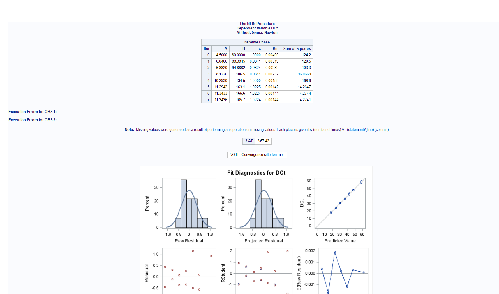
The model fits but refuses to go through the first points for some reason, which gives the following error message. 

This then leads to improper estimations of the parameters since it does not fit through the first points. It gives the first values as missing values. I feel like the answer is rather simple, but I cannot seem to grasp it. 

The data has been read properly, the table shows the correct values and plotting the data also gives the proper graphs.

Im running this on a SAS server running SAS studio 9.04.01M4P11092016 

[Rick_SAS]

I see. So the issue is that the procedure prints:

Execution Errors for OBS 1:

Execution Errors for OBS 2:

Note: Missing values were generated as a result of performing an operation on missing values. Each place is given by (number of times) AT (statement)/(line):(column).

Now I am puzzled, too. If Km and C are free parameters, then the expression (1-exp(-Km*Time))**C might not be a valid expression, since a**b is potentially undefined when a<0.

However, if you bound Km>0 and C>0, then the expression (1-exp(-Km*Time))**C ought to be a valid expression.

I will have to think about this...or maybe someone who uses PROC NLIN more than me knows the answer.  

[Rick_SAS · Accepted solution]

OK, I understand. The problem is not in evaluating the expression, it is in evaluating the derivative w.r.t C of the expression.

Recall that if a>0, then d/dx(a^x) = a^x*ln(a).  In your case, the derivative is w.r.t C and a=1-exp(-Km*Time).

The derivative is

d/dC(a^C) = a^C*ln(a)

which is only defined for a > 0.

You can avoid the point of discontinuity by modifying your PROC NLIN code:

proc nlin data=Have maxiter=2000;
parms A=2.5 Km=0.004 B=65 C=1;
bounds Km C >0;
expr = 1 - exp(-Km * Time);
if expr <= 0 then expr=1 - exp(-Km * 1e-12); /* nudge Time away from 0 */
model X = A + B * expr**C;
output out=IV p=yhat r=resid u95=upper parms= A Km B C;
run;
quit;

[GavinB]

Hi Rick,

This indeed seems to solve the problem for most of my parameters! Will look further into the ones that still give errors. Thanks for clearing things up.