- Home
- /
- Analytics
- /
- Forecasting
- /
- Re: proc arima transfer funtion
- RSS Feed
- Mark Topic as New
- Mark Topic as Read
- Float this Topic for Current User
- Bookmark
- Subscribe
- Mute
- Printer Friendly Page

- Mark as New
- Bookmark
- Subscribe
- Mute
- RSS Feed
- Permalink
- Report Inappropriate Content
Hello,
I have moderate background in time series analysis. I'm trying to do an intervention modeling using proc arima.
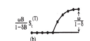
The model that I have postulated is an gradual permanent change such as shown below. See below for an example code. The problem that I'm facing is when I'm visualizing using ratio function using iml, I'm not able to get the appropriate effect. Any help in representing the gradual permanent change using transfer function in proc arima as well as visualizing using ratio function in proc arima would be greatly appreciated.
********************************************************************************************************************;
** Input Raw Data **;
********************************************************************************************************************;
data temp;
input cd @@;
datalines;
0 0 0 0 0 0.1 0.3 0.5
0.6 0.7 0.75 0.78 0.79 0.8
0.805 0.806 0.807 0.808 0.808
0.808 0.808
;
run;
********************************************************************************************************************;
** Create an indicator flag for Intervention **;
********************************************************************************************************************;
data temp;
set temp;
if _n_ > 5 then step = 1;
else step = 0;
run;
*****************************************************************************************************************;
** Identify the transfer function using cross correlation plot. **;
********************************************************************************************************************;
ods graphics on;
proc arima data=temp plots=all;
identify var=cd crosscorr = (step); /*Identify Transfer Function by CCF*/
estimate input = (/(1)step) method = ml outest = mm1; /*Estimate Model using Transfer Function Gradual Permanent Change*/
run;
ods graphics off;
********************************************************************************************************************;
** Extract Intervention for plotting **;
********************************************************************************************************************;
%let NUMLIST = 0.22;
%let DENLIST = -0.74;
%let nlags = 40;
proc iml;
Phi={&NUMLIST};
Theta={1 &DENLIST};
Psi=ratio(Theta,Phi,&NLAGS);
numLag=&NLAGS;
Lag=1:numLag;
Psi=Psi[1,1:numLag];
Y=Lag`||Psi`;
oname={'Lag' 'Psi'};
create temptransfer from Y[colname=oname];
append from Y;
close temptransfer;
run;
ods graphics on;
proc sgplot data=temptransfer;
vbar Lag / Response=Psi Stat=sum;
refline 0 / axis=y;
run;
ods graphics off;
Accepted Solutions

- Mark as New
- Bookmark
- Subscribe
- Mute
- RSS Feed
- Permalink
- Report Inappropriate Content
Hi.
You have created the effect correctly using you data step. This is seen by adding the following statement after the ESTIMATE statement and before the RUN in PROC ARIMA; FORECAST lead=0 printall;
As the forecast plot shows, your estimated a transfer function that generates a gradual build to a new status quo.
The IML portion of the code is outputting a data set that represents only the initial impact of the step and associated decay. That is, it is only capturing the effect of the first 1 in the step dummy. My IML is rusty, but the idea (and a brute forece way) would be to increment time; 1, 2, 3, 4, .... and then add effects corresponding to each interval and previous intervals. For example, looking at the Psi plot generated by your code, the effect, under a step intervention, at time 2 would by the effect at lag 2 + effect at lag 1. Effect at lag 3 = effect at lags 3 + 2 + 1. And so on.
Feel free to follow up and discuss details. My email is chip.wells@sas.com
- Mark as New
- Bookmark
- Subscribe
- Mute
- RSS Feed
- Permalink
- Report Inappropriate Content
Thank You very much.
.jpg")
Catch up on SAS Innovate 2026
Nearly 200 sessions are now available on demand in the Innovate Hub.
Watch Now →- Ask the Expert: R and SAS Working Seamlessly Together: Unlocking PROC R in Viya for Life Sciences | 11-Jun-2026
- Ask the Expert: Can Agents Reduce Planning Friction in CPG Supply Chains? | 16-Jun-2026
- Ask the Expert: Get Meaningful Results With New Features in SAS Customer Intelligence 360 | 25-Jun-2026
-
2 replies
-
07-25-2014 10:58 AM
-
2774 views
-
1 like
-
2 in conversation
-
