Hello,
I have moderate background in time series analysis. I'm trying to do an intervention modeling using proc arima.
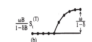
The model that I have postulated is an gradual permanent change such as shown below. See below for an example code. The problem that I'm facing is when I'm visualizing using ratio function using iml, I'm not able to get the appropriate effect. Any help in representing the gradual permanent change using transfer function in proc arima as well as visualizing using ratio function in proc arima would be greatly appreciated.
********************************************************************************************************************;
** Input Raw Data **;
********************************************************************************************************************;
data temp;
input cd @@;
datalines;
0 0 0 0 0 0.1 0.3 0.5
0.6 0.7 0.75 0.78 0.79 0.8
0.805 0.806 0.807 0.808 0.808
0.808 0.808
;
run;
********************************************************************************************************************;
** Create an indicator flag for Intervention **;
********************************************************************************************************************;
data temp;
set temp;
if _n_ > 5 then step = 1;
else step = 0;
run;
*****************************************************************************************************************;
** Identify the transfer function using cross correlation plot. **;
********************************************************************************************************************;
ods graphics on;
proc arima data=temp plots=all;
identify var=cd crosscorr = (step); /*Identify Transfer Function by CCF*/
estimate input = (/(1)step) method = ml outest = mm1; /*Estimate Model using Transfer Function Gradual Permanent Change*/
run;
ods graphics off;
********************************************************************************************************************;
** Extract Intervention for plotting **;
********************************************************************************************************************;
%let NUMLIST = 0.22;
%let DENLIST = -0.74;
%let nlags = 40;
proc iml;
Phi={&NUMLIST};
Theta={1 &DENLIST};
Psi=ratio(Theta,Phi,&NLAGS);
numLag=&NLAGS;
Lag=1:numLag;
Psi=Psi[1,1:numLag];
Y=Lag`||Psi`;
oname={'Lag' 'Psi'};
create temptransfer from Y[colname=oname];
append from Y;
close temptransfer;
run;
ods graphics on;
proc sgplot data=temptransfer;
vbar Lag / Response=Psi Stat=sum;
refline 0 / axis=y;
run;
ods graphics off;


.jpg")
