- Home
- /
- Analytics
- /
- Forecasting
- /
- Interpreting Results of PROC USM, ESM, and Performing ARIMA
- RSS Feed
- Mark Topic as New
- Mark Topic as Read
- Float this Topic for Current User
- Bookmark
- Subscribe
- Mute
- Printer Friendly Page
- Mark as New
- Bookmark
- Subscribe
- Mute
- RSS Feed
- Permalink
- Report Inappropriate Content
I am attempting to use SAS 9.4 to perform time series analysis so I can understand basic concepts. Despite heroic efforts I am utterly lost. I have literally spent 3 weeks going over hundreds of webpages, books, journals, and articles for well over 200 hours trying to understand the basics and feel no closer to my goal then when I began.
I have no idea what the SAS output is indicating and there is no straight answer or tutorial explaining how to read table or chart outputs to let me get on with it. Most of what is out there seems to assume you already know what time series elements are ...things such as level and damping factors ---and I do not. Or they are written by those more interested in showing off programming proweress instead of just creating very simple, easy to follow examples of the different situations that can arise with results. I don't want to create massive datasets and process them. I don't want to extrapolate between dates. That's irrelevant to my situation. Showing me an ACF and PACF plot is great when it deals with nicely lined up data but what if your plots come out like mine do. What then?
I just want to know - is my data seasonal? (I don't think so). Is it cyclical? (not on a regular cycle). Is there a trend? (not really). Are there diagnostics I can use on the data to build an appropriate ARIMA model? This work is driving me nuts.
Questions:
1. What models should I be using (UCM, ESM, ARIMA?) and what are the inputs I should be using to them?
- My data does not appear to have any regular cycle that I can see - it varies from 4 to 10 years. Now what?
- My data does not appear to have seasonality but I wanted to perform Simple Exponential Smoothing with seasonality and vary alpha
- the alpha in the statement appears to deal with confidence in the solution, not the alpha in this:YHATt|t+1 = alpha*Yt + alpha*(1-alpha)*Yt-1
- where can I vary the alpha - it seems to tell me my optimal value (usually either 0.001 or 0.999) but can I manually vary it somewhere?
2. What do the outputs tell me, eg.
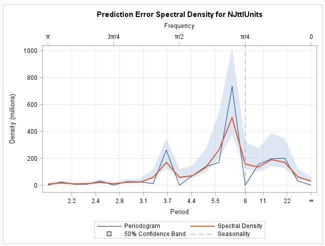
- What does a Spectral Density plot reveal about my data (the cycle length?) Where do I input that into a model?
- When I get a damping factor calculated, what exactly is it telling me? It's always about 0.88. And???
- What's the difference between a standardized ACF / PACF chart and the regular ACF/PACF ones?
- How do I interpret the ACF and PACF plots?
- What's IACF?
- What's a Smoothed Season State plot?
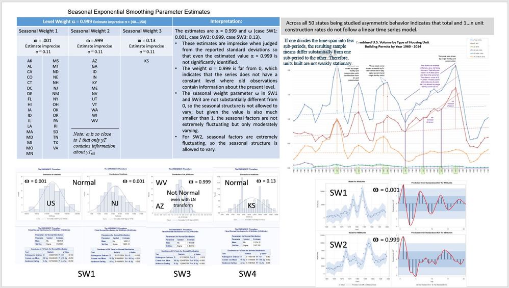
- What is "Level Weight" and "Seasonal Weight?" ...I assume SW is alpha ideal ~ either approx. 0 or approx. 1? What's the level weight mean? More basic, what is a level?
- How do you interpret the Final Estimates of the Free Parameters table?
- What are the meaning of "level" "slope" and "cycle" "damping factor" "period" and "error variance" in Component and Parameters
- Approx Pr > |t| is "good" when it is small, but what does it mean when it's almost 1?
- How do you use these results in ARIMA?
- In the Conditional Least Squares Estimation table, is the Pr>t that is small "good?" ... and therefore AR1,3 and MA1,3 are indicated - and how does that translate into the ARIMA(a,b,c) syntax? Is it a first difference so it's ARIMA(3,1,3)????????
I realize this is a bunch of questions. But I chose SAS and so I'm on my own. My class uses R but I have not because I prefer SAS. I have already spent a lot of money on books that don't help and am just blown away that it's so hard to get straight information on what I need to do to move on with my work. I don't want more phi's or psi's or theories. Just interpretations of actual results!
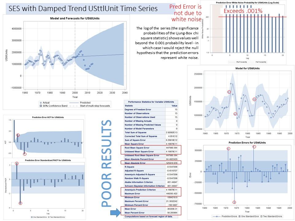
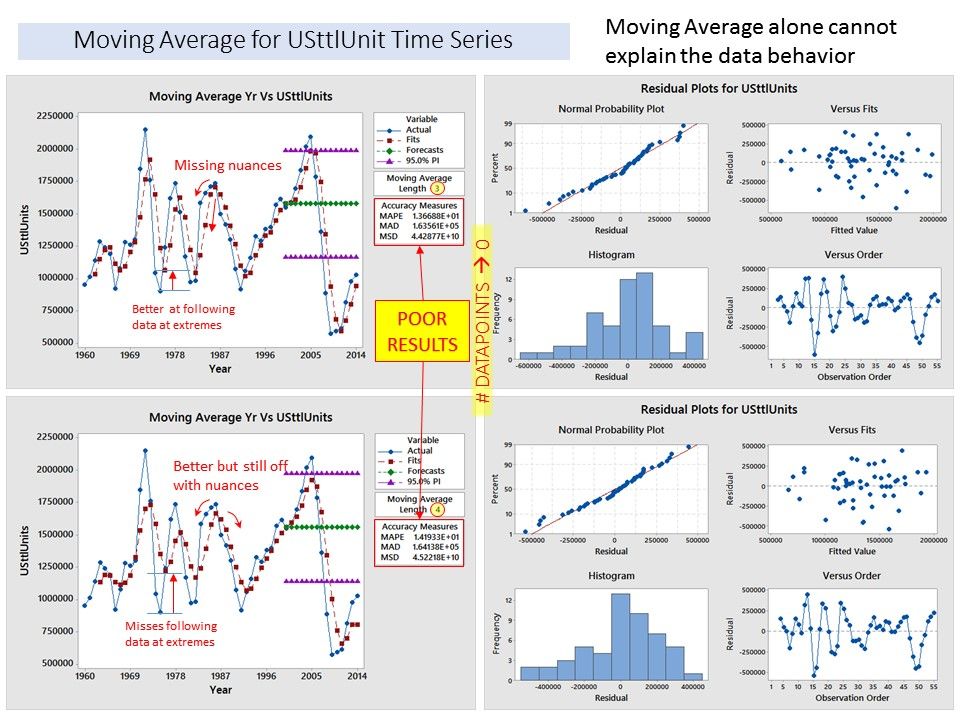
Can someone look at this data and what I've coded so far (attached in zip file) and try to help me along?
Accepted Solutions
- Mark as New
- Bookmark
- Subscribe
- Mute
- RSS Feed
- Permalink
- Report Inappropriate Content
I'll try to address the majority of your questions in a practical, applied approach in SAS, and keep theory to a minimum. In terms of which model to use to model your data, that's a question that varies greatly. Sometimes none of the models you listed are appropriate, sometimes more than one model can accurately forecast your series, and I'll try to address how you can tell. I'll try to highlight some of the questions you should be asking, and how to answer them using SAS software.
First, it appears YEAR is based on yearly increments. Because it's yearly, and not weekly, monthly, quarterly, etc., measuring seasonality isn't feasible. Before doing anything, it's a good idea to plot your series and check whether or not the series is white noise. Look at the ACF and White Noise plots to determine this.
proc timeseries data=<YOUR DATA SET> plots=(series corr);
id <TIMEID> interval=<TIMEIDINTERVAL>;
var <SERIES> / accumulate=none transform=none dif=0;
run;
Does your series contain significant autocorrelation? (Examine the ACF). Is the series White Noise? (Examine the White Noise plot). The ACF shows whether or not the series is autocorrelated with past lags, and the White Noise plot tells you if your series is pure random variation. The null hypothesis for the White Noise test is the series is white noise (i.e. the series is made up entirely of random variation and thus no need to use these modeling techniques).
If you have zero significant lags in the ACF (i.e. 0 lag(s) spiking above or below the confidence intervals), and you fail to reject the null hypothesis from the White Noise test, then the series is white noise. If you have significant spikes in the ACF, there is systematic variation that can be extracted from the series.
Next question: Do you have an input (exogenous) variable you plan to use to forecast the series? ARMAX, ARIMAX, and UCM can accomodate input variables. ESM cannot.
Within ESM there are seven different types of exponential smoothing models to choose from, all different variations of each other with different parameters (weights).
1. Simple (level)
2. Double (level)
3. Linear (level, trend)
4. Damped-Trend (level, trend, dampened)
5. Seasonal (level, seasonal)
6. Additive Winters (level, seasonal, trend)
7. Multiplicative Winters (level, seasonal, trend)
The Linear ESM only has a level and trend(slope) weight. Emperical evidence has shown long run forecasts using linear ESM over-forecast the trend as it tends to diminish over time. The damping weights allow the trend(slope) to diminish over time to help more accurately forecast the series. Imagine I created a poplar new widget that is selling 10 million units per week, and I want to forecast units per week over the next t weeks. At some point, that strong linear trend is probably going to level off, and the damping weight attempts to account for that, where the linear ESM would not.
Think of the level weight as where your series is on the y axis. As time changes, does the level of your series change? If so, is it due to trend? seasonality? both? pure random variation? Those are the questions ESM attempts to answer by capturing the effects of the specified model parameters of the specific model.
Notice additive winters and multiplicative winters both have the same three parameters. The difference is the multiplicative winters accounts for seasonal variation as the level of the series increases, whereas additive assumes constant seasonal variation. There's nothing wrong with running both and seeing which model gives you the best results. Because your model is in years, seasonality is an irrelevant parameter.
In terms of specifying parameter weights, SAS within PROC ESM calculates optimal smoothing weights that minimizes the residual sum of squares. To my knowledge, these can't be specified by the user. However, the larger the parameter, the more emphasis is placed on most recent values. An optimally chosen parameter close to 1 places much more emphasis on the most recent observation and decays more rapidly, whereas a weight close to zero places less interest in the most recent observation and is more equally spaced across the periods (i.e. decaying less rapidly).
After picking the appropriate ESM model, check the residuals of the model. For a good candidate model, the residuals should be iid White Noise. SAS will output residual diagnostics in the Results Viewer with a White Noise plot. If they aren't white noise, it means the model isn't capturing all of the systematic variation it could be. Perhaps a different model that allows for an input variable is appropriate (ARMAX, ARIMAX, UCM).
Regarding ARMA and ARIMA models, the first question is determining whether or not the series contains a unit root. Without getting too caught up in the math, you need to determine whether or not the series is stationary (i.e. exhibits a constant mean, constant variance, and constant covariance across the data points). The Augmented Dickey-Fuller test is helpful in determining this. The null hypothesis is your series contains a unit root (is not stationary). If you can reject the null at each specified lag, you can conclude the series is stationary. If your series is stationary, an ARMA model is appropriate, and you can model the series as is. If it isn't stationary, and just from the looks of it, USttlUnits doesn't appear stationary, try taking a first difference (Yt - Yt-1, Yt-1 - Yt-2, ... ) and modeling the first differenced data. This is where the I comes into play in ARIMA.
proc arima data=<DATA SET> plots (only)=(series(corr crosscorr) residual(corr normal) forecast(forecast forecastonly) );
identify var=USttlUnits(1) stationarity=(adf=(0 1)) scan esacf;
quit;
Use the estimate and forecast statements later to test and deploy models.
The next question is the systematic variation made up of autoregressive and/or moving average processes?
In PROC ARIMA, the SCAN and ESACF options help identify that for you. I use them all the time, as a series with both AR and MA terms can be tricky to identify by the ACF and PACF alone. There are ways to examine the ACF and PACF in determining this as well, but the SCAN and ESACF options are a good starting place.
To understand the difference between the ACF and PACF, consider this example. Suppose you examine the ACF and see a significant spike at lags 1 and 2. That means Yt is significantly autocorrelated with Yt-1 and Yt-2. It also means Yt-1 is significantly autocorrelated with Yt-2 and Yt-3. Similarly, Yt-3 is significantly autocorrelated with Yt-4 and Yt-5, and so on.
How do I know the significant autocorrelation between Yt and Yt-2 isn't just due to the fact that they're both significantly autocorrelated with Yt-1? Looking at the ACF, I don't. It's called the spillover effect. What I want to see is whether I have significant autocorrelation between Yt and Yt-2, holding constant the autocorrelation between Yt and Yt-1. That's what the PACF tells you. In a purely autoregressive model, the number of significant spikes in the PACF helps determine the number of AR parameters in the model. The opposite is true for purely moving average models.
Since moving average models are functions of past shocks (i.e. random errors assumed to be white noise and not autocorrelated with each other), the exact opposite is true. For pure moving average models, the ACF helps determine the number of significant moving average terms in the model.
You asked what inputs should you use in the model. If you're referring to AR and MA terms, refer to above. If you're referring to including an exogenous variable in an ARIMA, it's now called an ARIMAX model (X for exogenous input). Consider this... two series positively trending up over time. Are they related? How do you know? If they are, which influences which? Hybrid vehicle sales and bottled water consumption? Oil prices and gas prices? GDP and wild mountain lion sightings? The point is, just because they are autocorrelated doesn't mean they are related to each other. It's the whole "correlation does not imply causation" argument. Even if they are related, which causes which? And what is the relationship? These are questions the cross correlation function plot (CCF) can help determine. But before looking at the CCF, you've got to remove the autocorrelation from the input variable and "pre-whiten" the series. This will help determine the relationship and correctly specify the transfer function to use. SAS will automatically prewhiten for you in the ARIMA procedure.
You asked about the Final Estimates of the Free Parameters table... I'm assuming you are referring to UCM models. Based on the components specified, it tests whether the components are deterministic or stochastic. A p-value below alpha (by default at .05) suggests the component is stochastic. A p-value larger than alpha suggests the component is deterministic. If running a UCM, the Significance Analysis of Components (Based on the Final State) table will test whether or not each component is significant in the presence of other components in the model. This is one way to test whether your series has a significant trend component, cyclical component, and/or irregular component. Again, a seasonal component is off the table since it's yearly data.
In closing, the best applied forecasting book using SAS that I've ran across is Applied Data Mining for Forecasting Using SAS (http://www.sas.com/store/search.ep?keyWords=applied+data+mining+for+forecasting&submit=Search). It skips a lot of the hardcore math, explains the jargon in a way that makes sense, and jumps straight into examples of how to apply these models to real world data using SAS (with "non-jargon" interpretations).
- Mark as New
- Bookmark
- Subscribe
- Mute
- RSS Feed
- Permalink
- Report Inappropriate Content
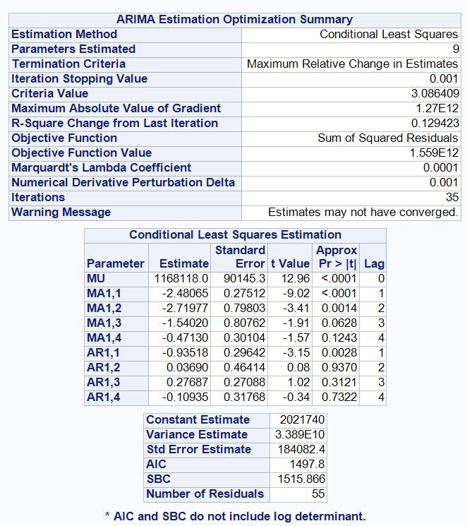
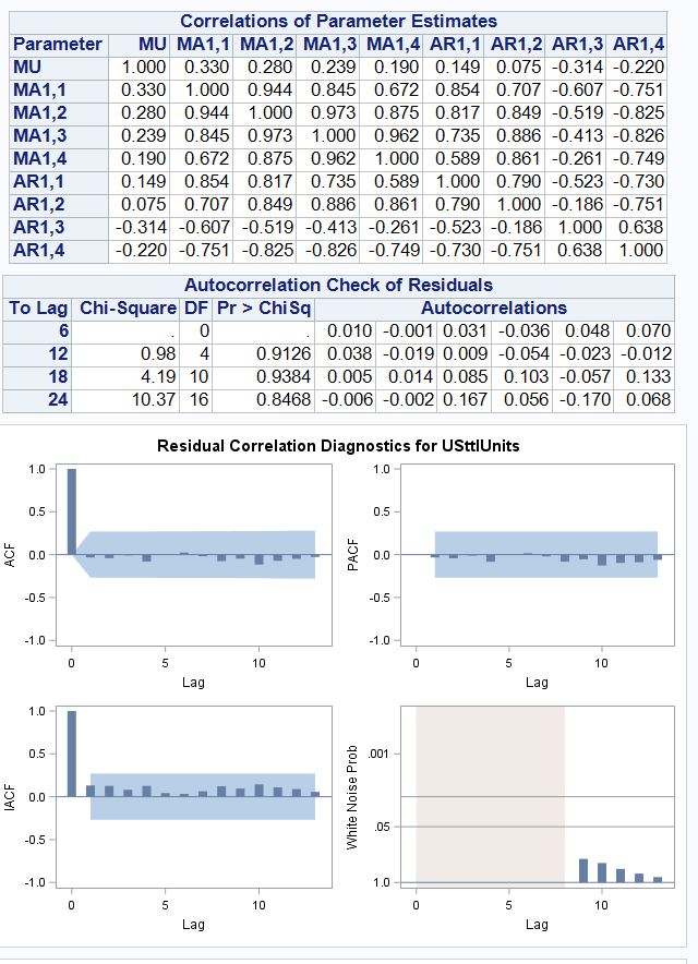
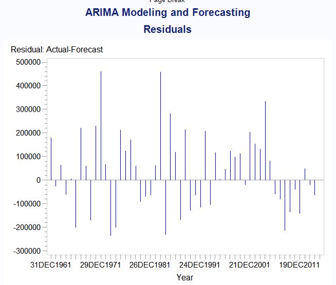
The ARIMA was run with dtUS (yT - yT-1). I am rerunning it as I originally did against the USttlUnits, VTttlUnits, and NJttlUnits.
The dtUS model resulted in the AR(1,3) and MA(1,3). I am confused what the lag 3 would be.
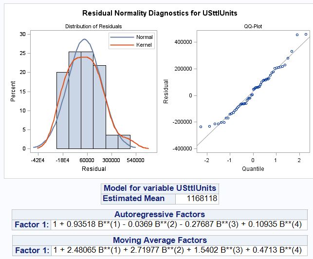
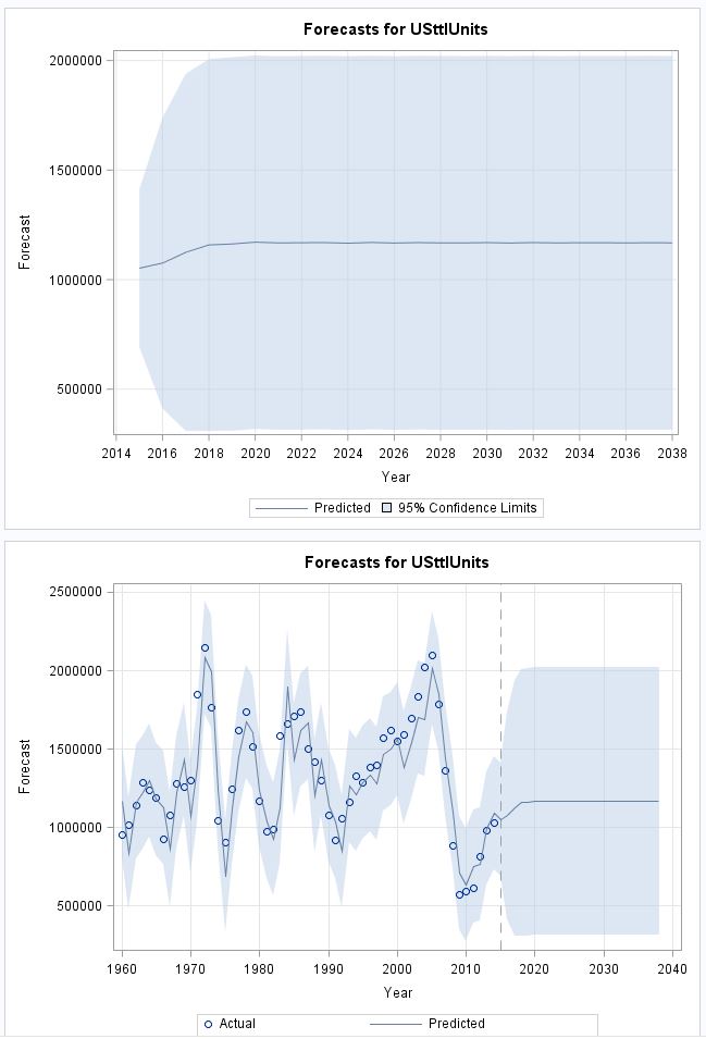
Here are the results for the USttlUnits ARIMA analysis.
- Mark as New
- Bookmark
- Subscribe
- Mute
- RSS Feed
- Permalink
- Report Inappropriate Content
I'll try to address the majority of your questions in a practical, applied approach in SAS, and keep theory to a minimum. In terms of which model to use to model your data, that's a question that varies greatly. Sometimes none of the models you listed are appropriate, sometimes more than one model can accurately forecast your series, and I'll try to address how you can tell. I'll try to highlight some of the questions you should be asking, and how to answer them using SAS software.
First, it appears YEAR is based on yearly increments. Because it's yearly, and not weekly, monthly, quarterly, etc., measuring seasonality isn't feasible. Before doing anything, it's a good idea to plot your series and check whether or not the series is white noise. Look at the ACF and White Noise plots to determine this.
proc timeseries data=<YOUR DATA SET> plots=(series corr);
id <TIMEID> interval=<TIMEIDINTERVAL>;
var <SERIES> / accumulate=none transform=none dif=0;
run;
Does your series contain significant autocorrelation? (Examine the ACF). Is the series White Noise? (Examine the White Noise plot). The ACF shows whether or not the series is autocorrelated with past lags, and the White Noise plot tells you if your series is pure random variation. The null hypothesis for the White Noise test is the series is white noise (i.e. the series is made up entirely of random variation and thus no need to use these modeling techniques).
If you have zero significant lags in the ACF (i.e. 0 lag(s) spiking above or below the confidence intervals), and you fail to reject the null hypothesis from the White Noise test, then the series is white noise. If you have significant spikes in the ACF, there is systematic variation that can be extracted from the series.
Next question: Do you have an input (exogenous) variable you plan to use to forecast the series? ARMAX, ARIMAX, and UCM can accomodate input variables. ESM cannot.
Within ESM there are seven different types of exponential smoothing models to choose from, all different variations of each other with different parameters (weights).
1. Simple (level)
2. Double (level)
3. Linear (level, trend)
4. Damped-Trend (level, trend, dampened)
5. Seasonal (level, seasonal)
6. Additive Winters (level, seasonal, trend)
7. Multiplicative Winters (level, seasonal, trend)
The Linear ESM only has a level and trend(slope) weight. Emperical evidence has shown long run forecasts using linear ESM over-forecast the trend as it tends to diminish over time. The damping weights allow the trend(slope) to diminish over time to help more accurately forecast the series. Imagine I created a poplar new widget that is selling 10 million units per week, and I want to forecast units per week over the next t weeks. At some point, that strong linear trend is probably going to level off, and the damping weight attempts to account for that, where the linear ESM would not.
Think of the level weight as where your series is on the y axis. As time changes, does the level of your series change? If so, is it due to trend? seasonality? both? pure random variation? Those are the questions ESM attempts to answer by capturing the effects of the specified model parameters of the specific model.
Notice additive winters and multiplicative winters both have the same three parameters. The difference is the multiplicative winters accounts for seasonal variation as the level of the series increases, whereas additive assumes constant seasonal variation. There's nothing wrong with running both and seeing which model gives you the best results. Because your model is in years, seasonality is an irrelevant parameter.
In terms of specifying parameter weights, SAS within PROC ESM calculates optimal smoothing weights that minimizes the residual sum of squares. To my knowledge, these can't be specified by the user. However, the larger the parameter, the more emphasis is placed on most recent values. An optimally chosen parameter close to 1 places much more emphasis on the most recent observation and decays more rapidly, whereas a weight close to zero places less interest in the most recent observation and is more equally spaced across the periods (i.e. decaying less rapidly).
After picking the appropriate ESM model, check the residuals of the model. For a good candidate model, the residuals should be iid White Noise. SAS will output residual diagnostics in the Results Viewer with a White Noise plot. If they aren't white noise, it means the model isn't capturing all of the systematic variation it could be. Perhaps a different model that allows for an input variable is appropriate (ARMAX, ARIMAX, UCM).
Regarding ARMA and ARIMA models, the first question is determining whether or not the series contains a unit root. Without getting too caught up in the math, you need to determine whether or not the series is stationary (i.e. exhibits a constant mean, constant variance, and constant covariance across the data points). The Augmented Dickey-Fuller test is helpful in determining this. The null hypothesis is your series contains a unit root (is not stationary). If you can reject the null at each specified lag, you can conclude the series is stationary. If your series is stationary, an ARMA model is appropriate, and you can model the series as is. If it isn't stationary, and just from the looks of it, USttlUnits doesn't appear stationary, try taking a first difference (Yt - Yt-1, Yt-1 - Yt-2, ... ) and modeling the first differenced data. This is where the I comes into play in ARIMA.
proc arima data=<DATA SET> plots (only)=(series(corr crosscorr) residual(corr normal) forecast(forecast forecastonly) );
identify var=USttlUnits(1) stationarity=(adf=(0 1)) scan esacf;
quit;
Use the estimate and forecast statements later to test and deploy models.
The next question is the systematic variation made up of autoregressive and/or moving average processes?
In PROC ARIMA, the SCAN and ESACF options help identify that for you. I use them all the time, as a series with both AR and MA terms can be tricky to identify by the ACF and PACF alone. There are ways to examine the ACF and PACF in determining this as well, but the SCAN and ESACF options are a good starting place.
To understand the difference between the ACF and PACF, consider this example. Suppose you examine the ACF and see a significant spike at lags 1 and 2. That means Yt is significantly autocorrelated with Yt-1 and Yt-2. It also means Yt-1 is significantly autocorrelated with Yt-2 and Yt-3. Similarly, Yt-3 is significantly autocorrelated with Yt-4 and Yt-5, and so on.
How do I know the significant autocorrelation between Yt and Yt-2 isn't just due to the fact that they're both significantly autocorrelated with Yt-1? Looking at the ACF, I don't. It's called the spillover effect. What I want to see is whether I have significant autocorrelation between Yt and Yt-2, holding constant the autocorrelation between Yt and Yt-1. That's what the PACF tells you. In a purely autoregressive model, the number of significant spikes in the PACF helps determine the number of AR parameters in the model. The opposite is true for purely moving average models.
Since moving average models are functions of past shocks (i.e. random errors assumed to be white noise and not autocorrelated with each other), the exact opposite is true. For pure moving average models, the ACF helps determine the number of significant moving average terms in the model.
You asked what inputs should you use in the model. If you're referring to AR and MA terms, refer to above. If you're referring to including an exogenous variable in an ARIMA, it's now called an ARIMAX model (X for exogenous input). Consider this... two series positively trending up over time. Are they related? How do you know? If they are, which influences which? Hybrid vehicle sales and bottled water consumption? Oil prices and gas prices? GDP and wild mountain lion sightings? The point is, just because they are autocorrelated doesn't mean they are related to each other. It's the whole "correlation does not imply causation" argument. Even if they are related, which causes which? And what is the relationship? These are questions the cross correlation function plot (CCF) can help determine. But before looking at the CCF, you've got to remove the autocorrelation from the input variable and "pre-whiten" the series. This will help determine the relationship and correctly specify the transfer function to use. SAS will automatically prewhiten for you in the ARIMA procedure.
You asked about the Final Estimates of the Free Parameters table... I'm assuming you are referring to UCM models. Based on the components specified, it tests whether the components are deterministic or stochastic. A p-value below alpha (by default at .05) suggests the component is stochastic. A p-value larger than alpha suggests the component is deterministic. If running a UCM, the Significance Analysis of Components (Based on the Final State) table will test whether or not each component is significant in the presence of other components in the model. This is one way to test whether your series has a significant trend component, cyclical component, and/or irregular component. Again, a seasonal component is off the table since it's yearly data.
In closing, the best applied forecasting book using SAS that I've ran across is Applied Data Mining for Forecasting Using SAS (http://www.sas.com/store/search.ep?keyWords=applied+data+mining+for+forecasting&submit=Search). It skips a lot of the hardcore math, explains the jargon in a way that makes sense, and jumps straight into examples of how to apply these models to real world data using SAS (with "non-jargon" interpretations).

2025 SAS Hackathon: There is still time!
Good news: We've extended SAS Hackathon registration until Sept. 12, so you still have time to be part of our biggest event yet – our five-year anniversary!
- Ask the Expert: How Do I Make a SAS Macro? | 09-Sep-2025
- Ask the Expert Webinar: Risque de Crédit : Modélisation, règles de décisions et Gouvernance | 16-Sep-2025
- SAS Bowl LIV, SAS and Generative AI | 17-Sep-2025
- Ask the Expert: PROC BGLIMM: The Smooth Transition to Bayesian Analysis | 18-Sep-2025
- Ask the Expert: Wie kann ich eine SAS 9.4 M9 Installation vorbereiten? | 19-Sep-2025
- SESUG 2025 on the SAS Campus, Sept. 22-24 | 22-Sep-2025
- Ask the Expert: Scaling Advanced Analytics Across the Enterprise With SAS Custom Analytics Framework | 23-Sep-2025
