Regression without P value?

[okla]

Hi, 

I have run a Stepwise regression model, and i am trying to interpret result, one of the Attributes, Addr_Type is with 0 degree of freedom and P value = ".", 

How should i interpret this? Would appreciate your help. Thanks. 

Here are my output... 

Type 3 Analysis of Effects

Wald
Effect DF Chi-Square Pr > ChiSq

Addr_Type 0 . .
Generation 7 102.7977 <.0001
IMP_LG10_If_Recency 1 184.6600 <.0001
OPT_Cnt_Issue_Agt 1 24.5667 <.0001
OPT_Cnt_RP 3 115.4793 <.0001
OPT_Entry_Ph_Age 3 11.7314 0.0084
OPT_Mosaic_Score 2 11.1377 0.0038
OPT_Patch_Age 3 151.7408 <.0001
OPT_TWP_UIP_Lifestyle 2 15.7572 0.0004
OPT_TWP_UIP_PA 1 15.5400 <.0001
OPT_TWP_W_Savings 2 26.2818 <.0001
Patch_Marital 5 16.5682 0.0054
Ph_Gender 4 20.2264 0.0005
ind_GECashflo 1 11.1497 0.0008
ind_GS 1 9.3346 0.0022
ind_LIssue_EQ_LSrvcng_Agt 1 22.9814 <.0001

Analysis of Maximum Likelihood Estimates

Standard Wald Standardized
Parameter DF Estimate Error Chi-Square Pr > ChiSq Estimate Exp(Est)

Intercept 1 -8.6528 23.3951 0.14 0.7115 0.000
Addr_Type 0. Unkno 1 -0.5979 0.2624 5.19 0.0227 0.550
Addr_Type HDB 1 -0.2478 0.0768 10.40 0.0013 0.781
Addr_Type Others 1 -0.3214 0.1351 5.66 0.0174 0.725
Addr_Type Private 0 0 . . . . .

OKLA. 

[Reeza]

Address type is categorical. If you have a categorical variable the reference level will not have estimates. 

[okla]

Hi, Thanks for your reply, but how does that explain my other categorical variables (e.g Generation/Gender/etc), they all have P value? 

Thanks. 

OKLA.

[Reeza]

They shouldn't...what parameterization method did you use?

[okla]

Hi, 

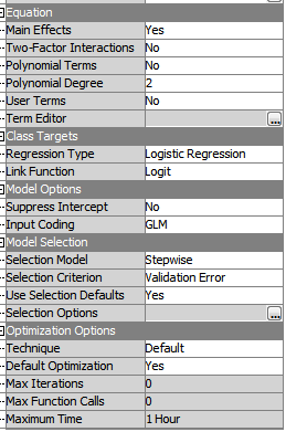
I am using SAS EM 12.1.

OKLA

[Reeza]

Change input coding from GLM to Reference and re-run. 

[Ksharp]

That is because the last level of Addr_Type is reference level, 
that means in real model there is not a variable corresponding to this level,
therefore you will see DF=0 P=. for this level.

If you want see non-missing value,you could change the reference level,like:
class Addr_Type(ref=first) ...........

[okla]

Hi, 

Thanks again for the help. Really appreciate it. 

I have tried 2 methods. 

Method 1 - Changing the GLM to Deviation in the Input Coding (EM12.1 only have either "GLM" or "Deviation"). Once i have changed it to Deviation, Addr_Type p value = 0.0012 now, but the reason why i used GLM at the first place is so that i have a reference variable to compare to, instead of compare to all the level in the same categorical (easier for me to explain to business users). 

Type 3 Analysis of Effects

Wald
Effect DF Chi-Square Pr > ChiSq

Addr_Type 3 15.8203 0.0012
Generation 7 102.7977 <.0001
IMP_LG10_If_Recency 1 184.6600 <.0001
OPT_Cnt_Issue_Agt 1 24.5667 <.0001
OPT_Cnt_RP 3 115.4793 <.0001
OPT_Entry_Ph_Age 3 11.7314 0.0084
OPT_Mosaic_Score 2 11.1377 0.0038
OPT_Patch_Age 3 151.7408 <.0001
OPT_TWP_UIP_Lifestyle 2 15.7572 0.0004
OPT_TWP_UIP_PA 1 15.5400 <.0001
OPT_TWP_W_Savings 2 26.2818 <.0001
Patch_Marital 5 16.5682 0.0054
Ph_Gender 4 20.2264 0.0005
ind_GECashflo 1 11.1497 0.0008
ind_GS 1 9.3346 0.0022
ind_LIssue_EQ_LSrvcng_Agt 1 22.9814 <.0001

Method 2 - I changed to use a different reference group (i.e. Addr_Type = Private as a reference group (in here is called REP_Addr_Type), the same P = . came out. 

Type 3 Analysis of Effects

Wald
Effect DF Chi-Square Pr > ChiSq

Generation 7 102.7977 <.0001
IMP_REP_LG10_If_Recency 1 184.6600 <.0001
OPT_Cnt_Issue_Agt 1 24.5667 <.0001
OPT_Cnt_RP 3 115.4793 <.0001
OPT_Entry_Ph_Age 3 11.7314 0.0084
OPT_Mosaic_Score 2 11.1377 0.0038
OPT_Patch_Age 3 151.7408 <.0001
OPT_TWP_UIP_Lifestyle 2 15.7572 0.0004
OPT_TWP_UIP_PA 1 15.5400 <.0001
OPT_TWP_W_Savings 2 26.2818 <.0001
Patch_Marital 5 16.5682 0.0054
Ph_Gender 4 20.2264 0.0005
REP_Addr_Type 0 . .
ind_GECashflo 1 11.1497 0.0008
ind_GS 1 9.3346 0.0022
ind_LIssue_EQ_LSrvcng_Agt 1 22.9814 <.0001

OKLA.