- RSS Feed
- Mark Topic as New
- Mark Topic as Read
- Float this Topic for Current User
- Bookmark
- Subscribe
- Mute
- Printer Friendly Page
- Mark as New
- Bookmark
- Subscribe
- Mute
- RSS Feed
- Permalink
- Report Inappropriate Content
I have some working code from a previous problem (thanks Rob). Which is an optimization problem that chooses the zonechoice such that the difference between initialzone and the zonechoice is minimal. Linearized solution:
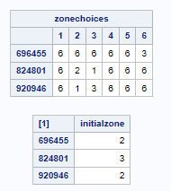
the dataset is for 3 items 824801, 696455, and 920946
data WORK.sMatrix;
Infile datalines delimiter='#';
input s initialzone var7 var8 var9 var10 var11 var12;
datalines;
824801#3#6#2#1#6#6#6
696455#2#6#6#6#6#6#3
920946#2#6#1#3#6#6#6
;
Run;

proc optmodel;
ods output PrintTable#3=expt3;

set SSET;
set JSET = 1..6;
num zonechoices {SSET, JSET};
num initialzone {SSET};

read data  sMatrix into SSET=[s] {j in JSET} <zonechoices[s,j]=col('Var'||(j+6))> initialzone;

print zonechoices initialzone;

var X {SSET, JSET} binary;
var Abs {SSET};

min Objective = (sum {s in SSET} Abs[s]) / (sum {s in SSET} initialzone[s]);

constraint OnceChoice {s in SSET}: sum {j in JSET} X[s,j] = 1;
constraint AbsCon1 {s in SSET}:Abs[s] >= sum {j in JSET} zonechoices[s,j]*X[s,j] - initialzone[s];
constraint AbsCon2 {s in SSET}:Abs[s] >= -sum {j in JSET} zonechoices[s,j]*X[s,j] + initialzone[s];

solve /*relaxint*/;
print X;

quit;
However, I want to now build upon this problem by imposing another rule. each zone in general is allowed to only have a certain amount of points.
a zone of 1 lower bound is 50 and the upper bound is 80
a zone of 2 lower bound is 40 and the upper bound is 60
a zone of 3 lower bound is 10 and the upper bound is 30
a zone of 6 is a dummy filler value that penalized at lower bound of 9999 and an upper bound of 9999
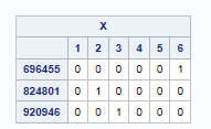
so the solution output by SAS (X is the solution matrix)
Proc OptModel indicates that the optimal solution is a zone 3, and a zone 3, and another zone 2
i.e
3 corresponds to 10 to 30 points
2 corresponds to 40 to 60 points
fig B) total 60 lower bound to 120
We can see that initially we have two zone 2's and a single zone 3 equating to a point range between 90 lower bound to 150 points upper bound (fig A).
this gives a difference of FigA and FigB is 30 and 30. I want to minimize this variance to the lower and upper bound as part of the optimal solution.
how can in incorporate this extra subproblem or constraint in this calculation?
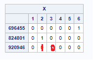
So a better solution that I came up with manually is :
which gives a point range difference of 10 lower and 20 upper
I was thinking use the midpoint of each range to set instead of using ranges altogether i.e for zone 1 would be 65 (midpoint). But then, I'm not sure how to add this extra minimization subproblem still...
thanks in advance from a struggling SAS user...
Accepted Solutions
- Mark as New
- Bookmark
- Subscribe
- Mute
- RSS Feed
- Permalink
- Report Inappropriate Content
You can treat the original objective as a primary objective and introduce a secondary objective that will break ties among solutions with the same primary objective value, by adding the following statements after the first solve:
set ZONES = {1,2,3,6};
num lb {ZONES} = [50, 40, 10, 9999];
num ub {ZONES} = [80, 60, 30, 9999];
num initialLb = sum {s in SSET} lb[initialzone[s]];
num initialUb = sum {s in SSET} ub[initialzone[s]];

num optimalObjectiveValue;
optimalObjectiveValue = Objective;
con ObjectiveCut:
	Objective <= optimalObjectiveValue;

var ErrorLb >= 0;
var ErrorUb >= 0;
min Objective2 = ErrorLb + ErrorUb;
impvar PointsLb = sum {s in SSET, j in JSET} lb[zonechoices[s,j]] * X[s,j];
impvar PointsUb = sum {s in SSET, j in JSET} ub[zonechoices[s,j]] * X[s,j];
con ErrorLbCon1:
	ErrorLb >= PointsLb - initialLb;
con ErrorLbCon2:
	ErrorLb >= -PointsLb + initialLb;
con ErrorUbCon1:
	ErrorUb >= PointsUb - initialUb;
con ErrorUbCon2:
	ErrorUb >= -PointsUb + initialUb;

solve;
print X;
print Objective;
print initialLb PointsLb ErrorLb;
print initialUb PointsUb ErrorUb;
print Objective2;
The resulting solution is the same as what you manually obtained:
- Mark as New
- Bookmark
- Subscribe
- Mute
- RSS Feed
- Permalink
- Report Inappropriate Content
Rob. Thank you so much! a perfect solution.
Catch up on SAS Innovate 2026
Dive into keynotes, announcements and breakthroughs on demand.
Explore Now →- Ask the Expert: Effective Methods for Working With SAS Date Values | 12-May-2026
- Club des utilisateurs SAS de Québec | 13-May-2026
- Ask the Expert: Welcome to SAS® Viya® | 14-May-2026
- Iowa SAS® Users Group’s 2026 One Day Conference | 15-May-2026
- WUSS Virtual Class: Introduction to R from a SAS Programmer’s Perspective | 15-May-2026
- WUSS Virtual Class: Asking Better Questions: The Art and Science of Survey Design | 19-May-2026
- Spring 2026 BC Health SAS User Group Meeting | 20-May-2026


