Multiple Optimization Functions within the same Proc OPTMODEL?

[SASAlex101]

I have some working code from a previous problem (thanks Rob). Which is an optimization problem that chooses the zonechoice such that the difference between initialzone and the zonechoice is minimal. Linearized solution: 

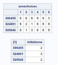
the dataset is for 3 items 824801, 696455, and 920946

data WORK.sMatrix;
Infile datalines delimiter='#';
input s initialzone var7 var8 var9 var10 var11 var12;
datalines;
824801#3#6#2#1#6#6#6
696455#2#6#6#6#6#6#3
920946#2#6#1#3#6#6#6
;
Run;

proc optmodel;
ods output PrintTable#3=expt3;

set SSET;
set JSET = 1..6;
num zonechoices {SSET, JSET};
num initialzone {SSET};

read data  sMatrix into SSET=[s] {j in JSET} <zonechoices[s,j]=col('Var'||(j+6))> initialzone;

print zonechoices initialzone;

var X {SSET, JSET} binary;
var Abs {SSET};

min Objective = (sum {s in SSET} Abs[s]) / (sum {s in SSET} initialzone[s]);

constraint OnceChoice {s in SSET}: sum {j in JSET} X[s,j] = 1;
constraint AbsCon1 {s in SSET}:Abs[s] >= sum {j in JSET} zonechoices[s,j]*X[s,j] - initialzone[s];
constraint AbsCon2 {s in SSET}:Abs[s] >= -sum {j in JSET} zonechoices[s,j]*X[s,j] + initialzone[s];

solve /*relaxint*/; 
print X;

quit;

However, I want to now build upon this problem by imposing another rule. each zone in general is allowed to only have a certain amount of points. 

a zone of 1 lower bound is 50 and the upper bound is 80

a zone of 2 lower bound is 40 and the upper bound is 60

a zone of 3 lower bound is 10 and the upper bound is 30

a zone of 6 is a dummy filler value that penalized at lower bound of 9999 and an upper bound of 9999

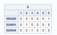
so the solution output by SAS (X is the solution matrix)

SASAlex101_6-1627075782990.png

SASAlex101_5-1627075775177.png

Proc OptModel indicates that the optimal solution is a zone 3, and a zone 3, and another zone 2

i.e

3 corresponds to 10 to 30 points

2 corresponds to 40 to 60 points

fig B) total 60 lower bound to 120

We can see that initially we have  two zone 2's  and a single zone 3 equating to a point range between 90 lower bound to 150 points upper bound (fig A).

this gives a difference of FigA and FigB is 30 and 30. I want to minimize this variance to the lower and upper bound as part of the optimal solution. 

how can in incorporate this extra subproblem or constraint in this calculation? 

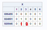
So a better solution that I came up with manually is :

SASAlex101_7-1627076260874.png

which gives a point range difference of 10 lower and 20 upper 

I was thinking use the midpoint of each range to set instead of using ranges altogether i.e for zone 1 would be 65 (midpoint). But then, I'm not sure how to add this extra minimization subproblem still...

thanks in advance from a struggling SAS user... 

[RobPratt · Accepted solution]

You can treat the original objective as a primary objective and introduce a secondary objective that will break ties among solutions with the same primary objective value, by adding the following statements after the first solve:

set ZONES = {1,2,3,6};
num lb {ZONES} = [50, 40, 10, 9999];
num ub {ZONES} = [80, 60, 30, 9999];
num initialLb = sum {s in SSET} lb[initialzone[s]];
num initialUb = sum {s in SSET} ub[initialzone[s]];

num optimalObjectiveValue;
optimalObjectiveValue = Objective;
con ObjectiveCut:
	Objective <= optimalObjectiveValue;

var ErrorLb >= 0;
var ErrorUb >= 0;
min Objective2 = ErrorLb + ErrorUb;
impvar PointsLb = sum {s in SSET, j in JSET} lb[zonechoices[s,j]] * X[s,j];
impvar PointsUb = sum {s in SSET, j in JSET} ub[zonechoices[s,j]] * X[s,j];
con ErrorLbCon1:
	ErrorLb >= PointsLb - initialLb;
con ErrorLbCon2:
	ErrorLb >= -PointsLb + initialLb;
con ErrorUbCon1:
	ErrorUb >= PointsUb - initialUb;
con ErrorUbCon2:
	ErrorUb >= -PointsUb + initialUb;

solve;
print X;
print Objective;
print initialLb PointsLb ErrorLb;
print initialUb PointsUb ErrorUb;
print Objective2;

The resulting solution is the same as what you manually obtained:

X
	1	2	3	4	5	6
696455	0	0	0	0	0	1
824801	0	1	0	0	0	0
920946	0	1	0	0	0	0

Objective
0.42857

initialLb	PointsLb	ErrorLb
90	100	10

initialUb	PointsUb	ErrorUb
150	170	20

Objective2
30

[SASAlex101]

Rob. Thank you so much! a perfect solution.