- Home
- /
- Programming
- /
- Graphics
- /
- How to fix the weights of this forest plot?
- RSS Feed
- Mark Topic as New
- Mark Topic as Read
- Float this Topic for Current User
- Bookmark
- Subscribe
- Mute
- Printer Friendly Page
- Mark as New
- Bookmark
- Subscribe
- Mute
- RSS Feed
- Permalink
- Report Inappropriate Content
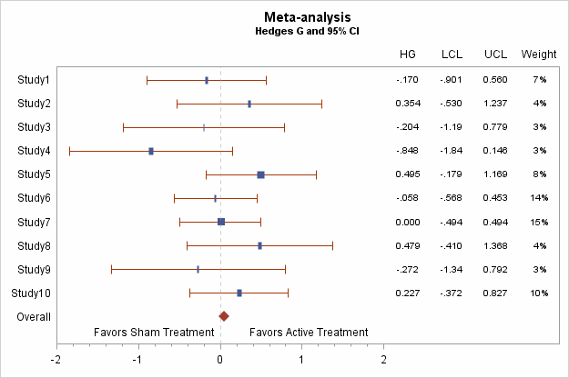
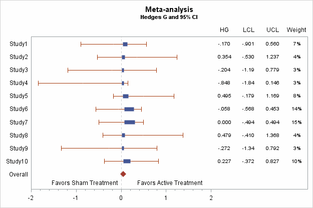
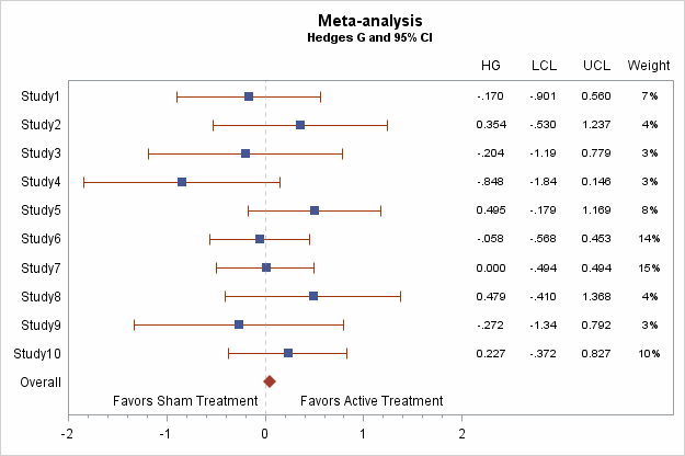
I've used the code from here to create a forest plot, and on another question someone kindly gave me some advice on how to change the scale to a non-log one. Unfortunately, I now have a new problem - the size of the weight boxes on the graph doesn't correspond to the pre-computed weights I've listed. Instead, the code is incorrectly calculating new weights/box sizes based on the hedge's g (referred to as 'odds ratio' in the code):
--e.g. 3% has two different sizes, 14% is smaller than 4%, etc
I've tried modifying the code to avoid that, but either:
1. It calculates the correct box size, but not anchored in the correct place:
2. It anchors the box in the correct place, but makes all the boxes a uniform size:
Is it possible to amend to the code to anchor the boxes in the right place and make them the correct size?
I've been modifying these lines:
   /* Compute marker width */
   x1=oddsratio / (10 ** (weight/2));
   x2=oddsratio * (10 ** (weight/2));
And this is the overall code I've been using:
data forest;
   input Study $1-18 grp OddsRatio LowerCL UpperCL Weight;
   format weight percent5. Q1 Q3 4.2 oddsratio lowercl uppercl 5.3;
   ObsId=_N_;
   OR='HG'; LCL='LCL'; UCL='UCL'; WT='Weight';
   if grp=1 then do;
      weight=weight*.01;
      Q1=OddsRatio-OddsRatio*weight;
      Q3=OddsRatio+OddsRatio*weight;
        lcl2=lowercl;
      ucl2=uppercl;
   end;
   else study2=study;
datalines;
Study1               1  -0.170 -0.901 0.560  7
Study2      	     1  0.354	-0.530	1.237 	4
Study3 	             1  -0.204	-1.186	0.779	3
Study4  	     1  -0.848	-1.842	0.146 	3
Study5	    	     1  0.495	-0.179	1.169   8
Study6               1 -0.058	-0.568	0.453  14
Study7               1  0.000	-0.494	0.494  15
Study8               1  0.479	-0.410	1.368 	4
Study9               1  -0.272	-1.335	0.792 	3
Study10              1	 0.227	-0.372	0.827  	10
Overall              2  0.0459 -0.1762 0.222 	 .
;
run;

proc sort data=forest out=forest2;
   by descending obsid;
run;

/* Add sequence numbers to each observation */
data forest3;
   set forest2 end=last;
   retain fmtname 'Study' type 'n';
   studyvalue=_n_;
   if study2='Overall' then study2value=1;
   else study2value = .;

/* Output values and formatted strings to data set */
   label=study;
   start=studyvalue;
   end=studyvalue;
   output;
   if last then do;
      hlo='O';
      label='Other';
   end;
run;

/* Create the format from the data set */
proc format library=work cntlin=forest3;
run;

/* Apply the format to the study values and remove Overall from Study column. */
/* Compute the width of the box proportional to weight in log scale. */
data forest4;
   format studyvalue study2value study.;
   drop fmtname type label start end hlo pct;
   set forest3 (where=(studyvalue > 0)) nobs=nobs;
   if studyvalue=1 then studyvalue=.;
   /* Compute marker width */
   x1=oddsratio / (10 ** (weight/2));
   x2=oddsratio * (10 ** (weight/2));

   /* Compute top and bottom offsets */
   if _n_ = nobs then do;
      pct=0.75/nobs;
      call symputx("pct", pct);
      call symputx("pct2", 2*pct);
      call symputx("count", nobs);
   end;
run;

ods listing close;
ods html image_dpi=100 path="." file='sgplotforest.html';
ods graphics / reset width=600px height=400px imagename="Forest_Plot_Vector" imagefmt=gif;

title "Meta-analysis       ";
title2 h=8pt 'Hedges G and 95% CI';

proc sgplot data=forest4 noautolegend;
   scatter y=study2value x=oddsratio / markerattrs=graphdata2(symbol=diamondfilled size=10);
   scatter y=studyvalue x=oddsratio / xerrorupper=ucl2 xerrorlower=lcl2 markerattrs=graphdata1(symbol=squarefilled size=0);
   vector x=x2 y=studyvalue / xorigin=x1 yorigin=studyvalue lineattrs=graphdata1(thickness=8) noarrowheads;
   scatter y=studyvalue x=or / markerchar=oddsratio x2axis;
   scatter y=studyvalue x=lcl / markerchar=lowercl x2axis;
   scatter y=studyvalue x=ucl / markerchar=uppercl x2axis;
   scatter y=studyvalue x=wt / markerchar=weight x2axis;
   refline 0 / axis=x lineattrs=(pattern=shortdash) transparency=0.5;
   inset '           Favors Sham Treatment'  / position=bottomleft;
   inset 'Favors Active Treatment'  / position=bottom;
   xaxis offsetmin=0 offsetmax=0.35 min=-2 max=2 minor display=(nolabel) ;
   x2axis offsetmin=0.7 display=(noticks nolabel);
   yaxis display=(noticks nolabel) offsetmin=0.1 offsetmax=0.05 values=(1 to &count by 1);
run;

ods html close;
ods listing;
Many thanks for any help!
Accepted Solutions
- Mark as New
- Bookmark
- Subscribe
- Mute
- RSS Feed
- Permalink
- Report Inappropriate Content
Hello @j4ne,
I think that's easy:
   /* Compute marker width */
    c=0.8; /* Factor to adjust absolute marker width */
   x1=oddsratio - c*weight;
   x2=oddsratio + c*weight;
As far as I see, only the relative marker widths have a meaning in the graph. Hence, we can introduce an arbitrary "scale factor" c to adjust the absolute marker width. I started with the "weight/2" from your code, i.e. c=0.5, but this seemed to be too small to distinguish between weights 3% and 4%. After removing "/2", i.e. with c=1, the markers were slightly longer than in your sample output with "correct box size". Therefore, I introduced variable c and set it to 0.8. But you can play around with this factor to obtain "optimal" box sizes.
- Mark as New
- Bookmark
- Subscribe
- Mute
- RSS Feed
- Permalink
- Report Inappropriate Content
Catch up on SAS Innovate 2026
Nearly 200 sessions are now available on demand with the SAS Innovate Digital Pass.
Explore Now →Learn how use the CAT functions in SAS to join values from multiple variables into a single value.
Find more tutorials on the SAS Users YouTube channel.
SAS Training: Just a Click Away
Ready to level-up your skills? Choose your own adventure.


