- Home
- /
- Programming
- /
- SAS Procedures
- /
- Re: how to find an asymptote from a scatter plot
- RSS Feed
- Mark Topic as New
- Mark Topic as Read
- Float this Topic for Current User
- Bookmark
- Subscribe
- Mute
- Printer Friendly Page

- Mark as New
- Bookmark
- Subscribe
- Mute
- RSS Feed
- Permalink
- Report Inappropriate Content
Hi,
I'm trying to determine the speed that a runner reaches at the end of a 3min all out effort. I have collected time and speed (at that given time) and when plotted on a scatter plot, it looks like it goes to an asymptote. Is there a procedure in SAS that can determine that asymptote speed? I wanted to use PROC NLIN but I don't know the function so I looked into PROC TRANSREG and the spline sometimes gives me the asymptote but sometimes it curves up at the end... Theoretically, it should be a smooth exponential decay or inverse curse from time zero to time (>3min).
here are my data...
| time(s) | speed (m/s) |
| 7.8 | 6.41 |
| 11.46 | 6.83 |
| 15.11 | 6.85 |
| 31.4 | 6.37 |
| 34.9 | 7.14 |
| 39 | 6.10 |
| 43.78 | 5.23 |
| 48.14 | 5.73 |
| 52.77 | 5.40 |
| 57.8 | 4.97 |
| 62.3 | 5.56 |
| 67.1 | 5.21 |
| 72.2 | 4.90 |
| 76.6 | 5.68 |
| 81.4 | 5.21 |
| 87.75 | 3.94 |
| 92.89 | 4.86 |
| 98.05 | 4.84 |
| 103.8 | 4.35 |
| 109.1 | 4.72 |
| 114.3 | 4.81 |
| 119.9 | 4.46 |
| 124.8 | 5.10 |
| 130.2 | 4.63 |
| 136.6 | 3.91 |
| 142 | 4.63 |
| 147.71 | 4.38 |
| 153.2 | 4.55 |
| 158.7 | 4.55 |
| 164.3 | 4.46 |
| 169.9 | 4.46 |
| 175.1 | 4.81 |
| 180.4 | 4.72 |
any help will be great!
thanks!
ming
Accepted Solutions

- Mark as New
- Bookmark
- Subscribe
- Mute
- RSS Feed
- Permalink
- Report Inappropriate Content
Try
proc nlin data=test;
parms Vo=2.5 a=-0.017 Vf=4.5;
model speed = Vo*exp(a*seconds) + Vf;
output out=outTest predicted=predSpeed;
run;
proc sgplot data=outTest noautolegend;
series x=seconds y=predSpeed;
scatter x=seconds y=speed;
yaxis min=0;
run;
Initial speed is Vo + Vf. Asymptotic speed is Vf.
Approx Approximate 95% Confidence
Parameter Estimate Std Error Limits
Vo 3.1430 0.3154 2.4989 3.7870
a -0.0176 0.00493 -0.0277 -0.00751
Vf 4.2795 0.2463 3.7765 4.7826
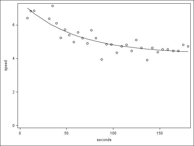
Seems to fit well...
PG
- Mark as New
- Bookmark
- Subscribe
- Mute
- RSS Feed
- Permalink
- Report Inappropriate Content
Try
proc nlin data=test;
parms Vo=2.5 a=-0.017 Vf=4.5;
model speed = Vo*exp(a*seconds) + Vf;
output out=outTest predicted=predSpeed;
run;
proc sgplot data=outTest noautolegend;
series x=seconds y=predSpeed;
scatter x=seconds y=speed;
yaxis min=0;
run;
Initial speed is Vo + Vf. Asymptotic speed is Vf.
Approx Approximate 95% Confidence
Parameter Estimate Std Error Limits
Vo 3.1430 0.3154 2.4989 3.7870
a -0.0176 0.00493 -0.0277 -0.00751
Vf 4.2795 0.2463 3.7765 4.7826
Seems to fit well...
PG
- Mark as New
- Bookmark
- Subscribe
- Mute
- RSS Feed
- Permalink
- Report Inappropriate Content
thanks for your help!
I tried it on another set of data with 4 data points, it didn't fit as well, but if I play around with the starting points for Vo, a, and Vf... sometimes I can get it to converge.
ming
- Mark as New
- Bookmark
- Subscribe
- Mute
- RSS Feed
- Permalink
- Report Inappropriate Content
Fitting a 3-parameter curve on 4 points doesn't give much freedom!
Given times T1-T4 and speeds S1-S4, you can try :
Vo=S1-S4, Vf=S4, a=-1.4/(T2+T3)
as starting values.
Good luck!
PG
.jpg")
Catch up on SAS Innovate 2026
Nearly 200 sessions are now available on demand with the SAS Innovate Digital Pass.
Explore Now →Learn the difference between classical and Bayesian statistical approaches and see a few PROC examples to perform Bayesian analysis in this video.

Find more tutorials on the SAS Users YouTube channel.
SAS Training: Just a Click Away
Ready to level-up your skills? Choose your own adventure.
-
3 replies
-
08-01-2013 12:52 PM
-
3753 views
-
0 likes
-
2 in conversation
-
