- Home
- /
- Programming
- /
- SAS Procedures
- /
- Re: Solve exponential equation
- RSS Feed
- Mark Topic as New
- Mark Topic as Read
- Float this Topic for Current User
- Bookmark
- Subscribe
- Mute
- Printer Friendly Page
- Mark as New
- Bookmark
- Subscribe
- Mute
- RSS Feed
- Permalink
- Report Inappropriate Content
Hi everyone. I need to solve this type of exponential equation: 
Accepted Solutions
- Mark as New
- Bookmark
- Subscribe
- Mute
- RSS Feed
- Permalink
- Report Inappropriate Content
Ah, I see. You want to each observation to represent a DIFFERENT equation and you want a DIFFERENT value of x for each observation. I had assumed you wanted a single value of x that would fit all the data in a least squares sense.
In your situation, each row represents an equation to be solved. Unfortunately, there is no reason to think that this equation has a solution for arbitrary values of D0, D1, and D2. For example, observations 9 and 28 in your data have
D0>0 and D1=D2. The equation becomes D2^x = 0 which has no solution. You might want to rethink (or explain) what you are trying to accomplish and describe where these numbers come. Clearly, some do not satisfy the equation.
For the ones that do, you can define
f(x) = D0^x - D1^x + D2^x
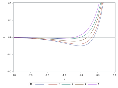
and solve for the root of f. Obviously f(0) > 0, so x=0 is never a root of f. A root is found in (-infinity, 0) or (0,infinity), depending on the values of the parameters. For the first few observation in your data set, the roots occur for x<0, as shown by the following graph. (If you know that x<0 always, that will simplify matters.)
data Have;
input D0 D1 D2;
ZERO = 0;
ID = _N_;
datalines;
22    7.07  22
22.02 7.28  19.03
21    10.05 19
19.03 8.06  19.03
17.03 8.94  15
;

data GraphIt;
set Have;
do x = -2 to 0 by 0.1;
   y = D0**x - D1**x + D2**x;
   output;
end;
run;

proc sgplot data=GraphIt;
   series x=x y=y / group=ID;
   refline 0 / axis=y;
   yaxis min=-0.2 max=0.2;
run;
Since you don't seem familiar with PROC NLIN, the simplest way to find the root of a univariate function in SAS is to use the FROOT function in SAS/IML
proc iml;
start Func(x) global (D0, D1, D2);
   return( D0**x - D1**x + D2**x );
finish;

use Have;
read all var {D0 D1 D2} into D;
close;

x = j(nrow(D),1);
do i = 1 to nrow(D);
   D0 = D[i,1]; D1 = D[i,2]; D2 = D[i,3];
   x[i] = froot("Func", {-2 0});
end;
print x;
If you don't have access to SAS/IML software, you'll have to learn how to use PROC NLIN:
options nonotes;
proc nlin data=Have noprint noitprint
          outest=PE(where=(_TYPE_="FINAL"));
   by ID;
   parms x -1;
   bounds x < 0;
   model ZERO = D0**x - D1**x + D2**x;
run;
options notes;

proc print data=PE noobs;
   var ID x;
run;
- Mark as New
- Bookmark
- Subscribe
- Mute
- RSS Feed
- Permalink
- Report Inappropriate Content
Check PROC NLIN to fit an non-linear model.
Or Check FROOT() function in IML documentation.
Or post it at OR forum, @RobPratt might use OR code to solve it .
And @Rick_SAS has wrote many blog to solve such kind of question.
https://blogs.sas.com/content/iml/2015/06/08/fit-circle.html
- Mark as New
- Bookmark
- Subscribe
- Mute
- RSS Feed
- Permalink
- Report Inappropriate Content
This looks like a job for PROC NLIN. You need a variable for the response, which is constantly zero. The following statements assume that the data for D0, D1, and D2 are in the data set MyData. I create a new data set called Have that appends a columns of zeros to use as the response. I also assume that you are interested in x > 0.
data Have;
set MyData;
ZERO = 0;
run;

proc nlin data=Have;
   parms x 1;
   bounds 0 < x;
   model ZERO = D0**x - D1**x + D2**x;
run;
- Mark as New
- Bookmark
- Subscribe
- Mute
- RSS Feed
- Permalink
- Report Inappropriate Content
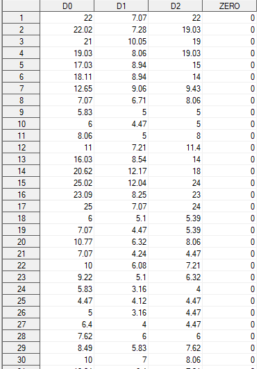
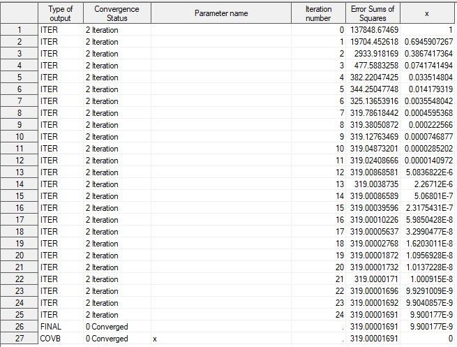
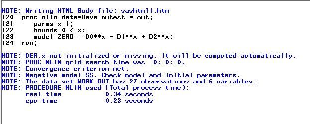
I need to count x for each set of D0, D1 and D2. But I don't actually understand what does the code that you provided. I attach screenshots of my dataset and result.
- Mark as New
- Bookmark
- Subscribe
- Mute
- RSS Feed
- Permalink
- Report Inappropriate Content
I don't know what "count x for each set of D0, D1 and D2" means. The procedure fits a nonlinear regression model that finds the value of x that best fits the model to the entire set of observations. The SAS documentation gives an overview of PROC NLIN.
If you don't want to see the iteration history, you can use the NOITPRINT option on the PROC NLIN statement. The important line in the output is observation 26 (WHERE=(_TYPE_="FINAL")), which says that the best fit of the model to your data is to make x a very small positive number (essentially 0). When x=0, the equation reduces to 1-1+1=0 + eps, where eps is normal random error. This result seems to indicate that this model is not a good fit to the data.
- Mark as New
- Bookmark
- Subscribe
- Mute
- RSS Feed
- Permalink
- Report Inappropriate Content
"Count x for each set of D0,D1 and D2" means, for instance: if D0 = 25, D1=24 and D2 = 7 (obs N 17 in my dataset) then I have 25^x - 24^x - 7^x = 0. For this example x = 2, because 25^2 - 24^2 - 7^2 = 625 - 576 - 49 = 0.
Exapmple №2: if D0 = 4.5, D1 = 4 and D2 = 3 then x =3, because 4.5^3 - 4^3 - 3^3 = 91 - 64 - 27 = 0.
And I understand that I should look on observation WHERE=(_TYPE_="FINAL").
- Mark as New
- Bookmark
- Subscribe
- Mute
- RSS Feed
- Permalink
- Report Inappropriate Content
Ah, I see. You want to each observation to represent a DIFFERENT equation and you want a DIFFERENT value of x for each observation. I had assumed you wanted a single value of x that would fit all the data in a least squares sense.
In your situation, each row represents an equation to be solved. Unfortunately, there is no reason to think that this equation has a solution for arbitrary values of D0, D1, and D2. For example, observations 9 and 28 in your data have
D0>0 and D1=D2. The equation becomes D2^x = 0 which has no solution. You might want to rethink (or explain) what you are trying to accomplish and describe where these numbers come. Clearly, some do not satisfy the equation.
For the ones that do, you can define
f(x) = D0^x - D1^x + D2^x
and solve for the root of f. Obviously f(0) > 0, so x=0 is never a root of f. A root is found in (-infinity, 0) or (0,infinity), depending on the values of the parameters. For the first few observation in your data set, the roots occur for x<0, as shown by the following graph. (If you know that x<0 always, that will simplify matters.)
data Have;
input D0 D1 D2;
ZERO = 0;
ID = _N_;
datalines;
22    7.07  22
22.02 7.28  19.03
21    10.05 19
19.03 8.06  19.03
17.03 8.94  15
;

data GraphIt;
set Have;
do x = -2 to 0 by 0.1;
   y = D0**x - D1**x + D2**x;
   output;
end;
run;

proc sgplot data=GraphIt;
   series x=x y=y / group=ID;
   refline 0 / axis=y;
   yaxis min=-0.2 max=0.2;
run;
Since you don't seem familiar with PROC NLIN, the simplest way to find the root of a univariate function in SAS is to use the FROOT function in SAS/IML
proc iml;
start Func(x) global (D0, D1, D2);
   return( D0**x - D1**x + D2**x );
finish;

use Have;
read all var {D0 D1 D2} into D;
close;

x = j(nrow(D),1);
do i = 1 to nrow(D);
   D0 = D[i,1]; D1 = D[i,2]; D2 = D[i,3];
   x[i] = froot("Func", {-2 0});
end;
print x;
If you don't have access to SAS/IML software, you'll have to learn how to use PROC NLIN:
options nonotes;
proc nlin data=Have noprint noitprint
          outest=PE(where=(_TYPE_="FINAL"));
   by ID;
   parms x -1;
   bounds x < 0;
   model ZERO = D0**x - D1**x + D2**x;
run;
options notes;

proc print data=PE noobs;
   var ID x;
run;
- Mark as New
- Bookmark
- Subscribe
- Mute
- RSS Feed
- Permalink
- Report Inappropriate Content
Thank you very much. I managed to solve my problem using your article https://blogs.sas.com/content/iml/2014/02/05/find-the-root-of-a-function.html
Here there is my code. Also I have a problem with adding z to a dataset.
%macro lambda;

%do i = 1 %to &n_obs.;

  data _null_;
    set have (where = (a = &i.));
    call symput("d_0",d0);
    call symput("d_1",db);
    call symput("d_2",dt);
  run;

  proc iml;
    start Func(x);
      return( &d_0.**x - &d_1.**x - &d_2.**x );
    finish;

    intervals = {-10   10};
    z = froot("Func", intervals);
  print z;
  quit;

%end;
%mend lambda;
Catch up on SAS Innovate 2026
Nearly 200 sessions are now available on demand with the SAS Innovate Digital Pass.
Explore Now →Learn the difference between classical and Bayesian statistical approaches and see a few PROC examples to perform Bayesian analysis in this video.
Find more tutorials on the SAS Users YouTube channel.
SAS Training: Just a Click Away
Ready to level-up your skills? Choose your own adventure.

