- Home
- /
- Programming
- /
- SAS Procedures
- /
- Re: Saving p-values
- RSS Feed
- Mark Topic as New
- Mark Topic as Read
- Float this Topic for Current User
- Bookmark
- Subscribe
- Mute
- Printer Friendly Page
- Mark as New
- Bookmark
- Subscribe
- Mute
- RSS Feed
- Permalink
- Report Inappropriate Content
Hi,
I am trying to do a Monte Carlo simulation of ANCOVA. I generated random variables and simulated data from regressions models below. x is a covariate, g is a grouping variable (0 for a control group, 1 for a treatment group), y is a dependent variable. I am manipulating coefficients. In this syntax, I set the treatment effect on y to be 0, the treatment effect on x to be 0.6, and the effect of x on y to be 1. I also set the number of samples to be 1000 and the sample size to be 800 (about a half being a treatment group).
data MC (drop=i);
call streaminit(12345678);
do sampleID = 1 to 1000;
  do i = 1 to 800;
    g = rand("Bernoulli", 0.5);
    x = 0.6*g + rand("Normal");
    y = 1*x + 0*g + rand("Normal");
    output;
  end;
end;
run;
So, after that, I need to test the effect of g on y in each of 1000 samples. I wrote this syntax:
proc glm data = MC;
  BY sampleID;
  class g;
  model y = g;
run;
It works but the problem is that I need only p values (for F values) from the output to count how many were less then .05 (which will serve as an estimate of Type I error rate). So, I can't figure out how to put these p-values in a data set, an array, or something like that (extracting p-values by hand for 1000 samples is not an option...).
I would very much appreciate any help and/or feedback. Thank you.
Accepted Solutions
- Mark as New
- Bookmark
- Subscribe
- Mute
- RSS Feed
- Permalink
- Report Inappropriate Content
Here is how to do the counting (for effect g):
proc glm data = MC outstat=myStat noprint;
  BY sampleID;
  class g;
  model y = g x / ss3;
run;

proc sql;
select
    sum(prob<0.05) as nb_5pct,
    count(prob) as nb_sample,
    sum(prob<0.05) / count(prob) as prop_5pct
from myStat
where _SOURCE_ = "g";
quit;
- Mark as New
- Bookmark
- Subscribe
- Mute
- RSS Feed
- Permalink
- Report Inappropriate Content
Start with:
proc glm data = MC outstat=myStat noprint;
  BY sampleID;
  class g;
  model y = g x / ss3;
run;
- Mark as New
- Bookmark
- Subscribe
- Mute
- RSS Feed
- Permalink
- Report Inappropriate Content
Thank you! Now I have one table with all p values!
Last question -- how now to count p that less than 0.05? I though I can use myStat now as a data set and PROB as a variable so that I could simply count through the if statement -- but that doesn't seem to work...
Thank you in advance.
- Mark as New
- Bookmark
- Subscribe
- Mute
- RSS Feed
- Permalink
- Report Inappropriate Content
@Amanda_Lemon wrote:
Thank you! Now I have one table with all p values!
Last question -- how now to count p that less than 0.05? I though I can use myStat now as a data set and PROB as a variable so that I could simply count through the if statement -- but that doesn't seem to work...
Thank you in advance.
What does that code look like, that logic should work fine.
- Mark as New
- Bookmark
- Subscribe
- Mute
- RSS Feed
- Permalink
- Report Inappropriate Content
Here is how to do the counting (for effect g):
proc glm data = MC outstat=myStat noprint;
  BY sampleID;
  class g;
  model y = g x / ss3;
run;

proc sql;
select
    sum(prob<0.05) as nb_5pct,
    count(prob) as nb_sample,
    sum(prob<0.05) / count(prob) as prop_5pct
from myStat
where _SOURCE_ = "g";
quit;
- Mark as New
- Bookmark
- Subscribe
- Mute
- RSS Feed
- Permalink
- Report Inappropriate Content
Thank you so much!! It works!
- Mark as New
- Bookmark
- Subscribe
- Mute
- RSS Feed
- Permalink
- Report Inappropriate Content
An unrelated follow-up question. When I simulate the binary variable g, I use the Bernoulli distribution. I want the two groups to be equal, so I thought that setting the probability to 0.5 will do that. But it produces approximate splits in half (like, 423 and 377). I know I can just assign 0 to g for i from 1 to 400 and 1 to g for i from 401 to 800. But is there a way to _randomly_ assign 0 and 1 to g but have the groups precisely equal (400 and 400)?
Thanks again for your help.
data MC (drop=i);
call streaminit(12345678);
do sampleID = 1 to 1000;
  do i = 1 to 800;
    g = rand("Bernoulli", 0.5);
    x = 0.6*g + rand("Normal");
    y = 1*x + 0*g + rand("Normal");
    output;
  end;
end;
run;- Mark as New
- Bookmark
- Subscribe
- Mute
- RSS Feed
- Permalink
- Report Inappropriate Content
There is no advantage in having random g values, as far as I can tell. But if you want, you can do:
data temp (drop=i);
call streaminit(12345678);
do sampleID = 1 to 1000;
    do g = 0, 1;
        do i = 1 to 400;
            rnd = rand("Uniform");
            x = 0.6*g + rand("Normal");
            y = 1*x + 0*g + rand("Normal");
            output;
            end;
        end;
    end;
run;

proc sort data=temp out=mc(drop=rnd);
by sampleId rnd;
run;
(untested)
- Mark as New
- Bookmark
- Subscribe
- Mute
- RSS Feed
- Permalink
- Report Inappropriate Content
- Mark as New
- Bookmark
- Subscribe
- Mute
- RSS Feed
- Permalink
- Report Inappropriate Content
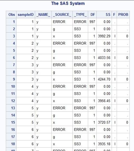
I ran into another problem... Everything works just fine when I simulate a normal distribution but when I changed it to a truncated normal distribution, the PROC GLM statement stopped working... (data are simulated fine). When I print the GLM results, it shows that SS for g were not computed (see the screenshot). Why is that? Thank you in advance.
data MC (keep = x y g sampleID);
Fa = cdf('Normal', -6, 0, 1); /* for a = -6 */
Fb = cdf('Normal', 6, 0, 1); /* for b = 6 */
call streaminit(12345678);
do sampleID = 1 to 1000;
 do g = 0, 1;
  do i = 1 to 500;
    v = Fa + (Fb-Fa)*rand('Uniform'); /* V ~ U(F(a), F(b)) */
    x = 0*g + quantile('Normal', v, 0, 1); /* truncated normal on [a,b] */
    y = 1*x + 0*g + quantile('Normal', v, 0, 1);
    output;
  end;
 end;
end;
run;
proc glm data = MC outstat=myStat noprint;
  BY sampleID;
  class g;
  model y = g x / ss3;
run;
proc print data = myStat;
run;- Mark as New
- Bookmark
- Subscribe
- Mute
- RSS Feed
- Permalink
- Report Inappropriate Content
The problem stems from the fact that y = 2*x in all of your simulated observations. To replicate the structure of your previous simulation you would need:
    v = Fa + (Fb-Fa)*rand('Uniform'); /* V ~ U(F(a), F(b)) */
    w = Fa + (Fb-Fa)*rand('Uniform'); /* W ~ U(F(a), F(b)) */
    x = 0*g + quantile('Normal', v, 0, 1); /* truncated normal on [a,b] */
    y = 1*x + 0*g + quantile('Normal', w, 0, 1);
- Mark as New
- Bookmark
- Subscribe
- Mute
- RSS Feed
- Permalink
- Report Inappropriate Content
Learn the difference between classical and Bayesian statistical approaches and see a few PROC examples to perform Bayesian analysis in this video.
Find more tutorials on the SAS Users YouTube channel.
SAS Training: Just a Click Away
Ready to level-up your skills? Choose your own adventure.


