- Home
- /
- Programming
- /
- SAS Procedures
- /
- Re: Calculating mean + sd on non-normal data
- RSS Feed
- Mark Topic as New
- Mark Topic as Read
- Float this Topic for Current User
- Bookmark
- Subscribe
- Mute
- Printer Friendly Page
- Mark as New
- Bookmark
- Subscribe
- Mute
- RSS Feed
- Permalink
- Report Inappropriate Content
Hi all
Currently at the company I work for, we use benchmarks of 'subjects' (I call it 'subjects' because of anonimity reasons) in order to discover subjects with 'unusual behaviour'. Basically what we do is: we have a set of subjects with a 'score' on a 'risk'. We want to discover the 'highest scorers' (hence we use benchmark) in order to 'further analyze them'.
Until now, we have worked with percentiles in order to define the ‘subjects to further analyse’. Let’s say we have 150 subjects with a score between 0 and 1 (percentage), ranked from high to low. What we did until now is to say: let’s further analyse all the subjects above the 90th percentile = the 10% highest scorers. As you all know, this method doesn’t account for the actual scores, the mean of the scores or the spread within the scores. If I have 150 subjects, which score relatively the same on a risk, except for the top 3, which score very high, I don’t want to further investigate the top 10% (15 subjects), but only the top 3, right?
Therefore we are now looking for a method better than percentiles to determine the ‘highest scorers’. FYI, we don’t bother with the lowest scorers (yet). One method we are thinking of is of course the use of the mean + X*standard deviations. Doing so, the subjects who fall outside our predefined upper range, defined as 1,28 (=upper 10%) or 1,64 (=upper 5%) or 1,96 (=upper 2,5%) times the standard deviation, will be flagged as ‘to be further analyzed’.
So far, so good. This looks to me like a solid method to determine the highest scorers, while taking into account the mean and the spread in the data.
As the title suggests though, most of the ‘risks’ we analyse, contain data which is not normally distributed. That still doesn’t have to be a problem, since data can be transformed in order to become normally distributed. I know of different kinds of transformation, according to Tukey’s ladder of transformation. After transformation I can calculate mean and upper range and then transform the data back to the original values in order to determine who are my subjects of interest. This sounds like a solid method to me, right? Transformation --> calculation --> back-transformation, is what is always used in science, as far as I know.
Now we come to the main questions of this discussion:
- How do I determine if my data is normally distributed after transformation?
- What if my data is still not (perfectly) normally distributed even after transformation? Can I still use the method of mean + X*standard deviation in order to determine which subjects to further analyse?
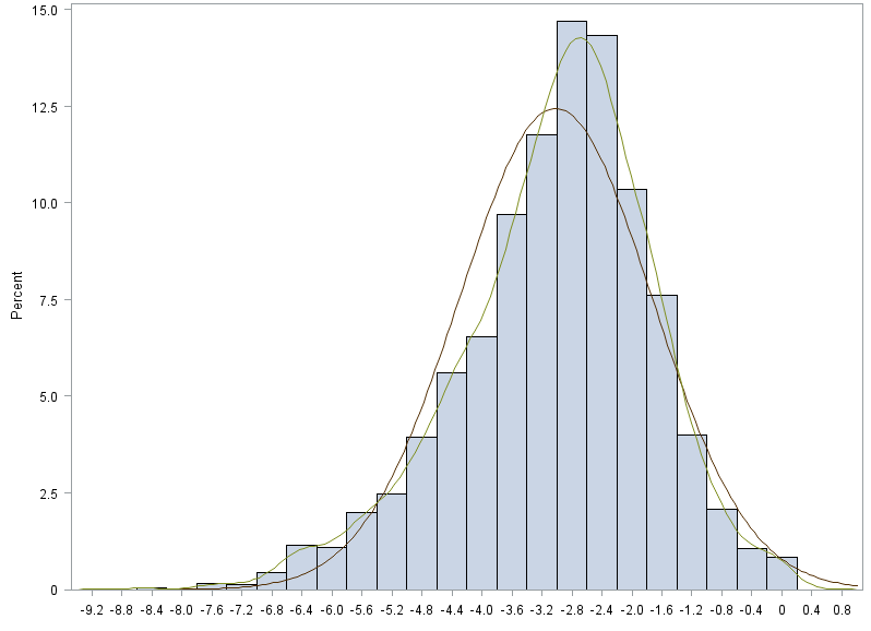
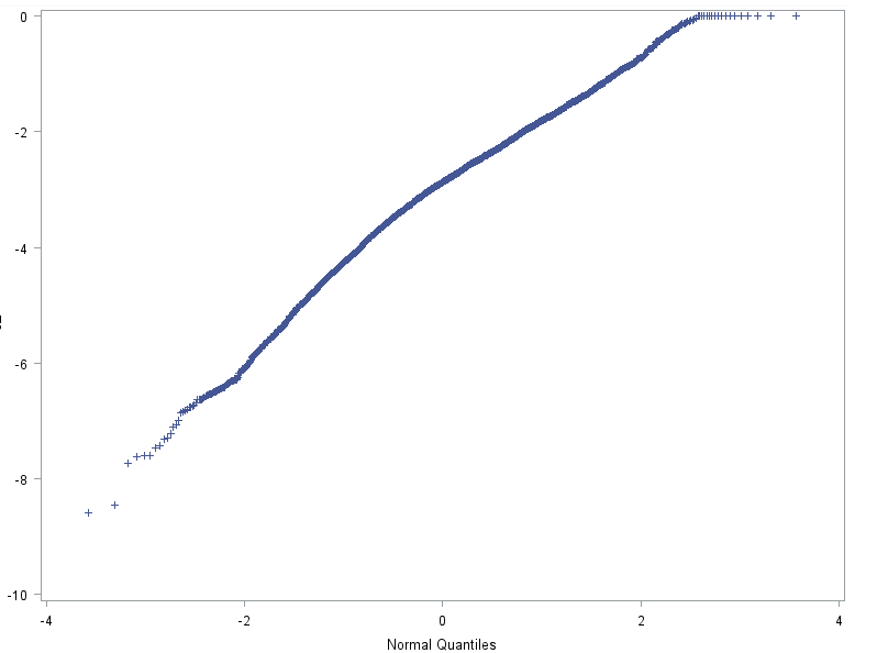
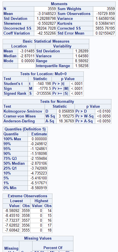
I have attached 3 files in order to show how I determine if my data is (somewhat) normally distributed. The data used to generate the 3 files, is already ln-transformed (log(x) in SAS, not log10(x)).
The first picture shows the result the univariate procedure.
In this output I look at different things:
- Skewness and kurtosis:
- If skewness is between -1 and +1, it suggests to me a normal distribution
- If kurtosis is < 1, it suggests to me a normal distribution.
- Mean and median
- If mean is approximately the same as the median, it suggests to me a normal distribution
- Tests for normality
- If the tests are NOT significant, it suggests to me a normal distribution.
Then I look at the histogram:
- If it ‘looks like’ a normal distribution, it suggests to me a normal distribution.
Then I look at the QQplot:
- If it is almost totally a straight line, it suggests to me a normal distribution.
Based on the files I attached, I would decide that my ln-transformed data is distributed normally enough in order to do my mean + X*sd calculations.
I realize that most of the judgments I make are ‘arbitrary’, except for the tests of normality. The only non-arbitrary measures of normality (the tests for normality) reject the hypothesis of normally distributed data, and still I would conclude that my data is distributed normally enough, based on what I ‘see’. Hence I am here asking for help on the matter.
1) Is my method of determining normality of the transformed data appropriate? If not, how can I best judge if my data is normally distributed?
2) What other transformations of tricks are there to get normally distributed data, of the ‘regular’ methods don’t work?
3) If I still do mean + X*sd calculations on not perfectly normal data, what are the consequences of this? And then specifically, what are the consequences of this looking at my initial questions, i.e. determine the high scorers / subjects of interest?
Finally, do I REALLY require (perfectly) normally distributed data in order to select my ‘subjects of interest’ with the method of mean + X*sd?


- Mark as New
- Bookmark
- Subscribe
- Mute
- RSS Feed
- Permalink
- Report Inappropriate Content
I took the liberty of copying out your attached file:
Currently at the company I work for, we use benchmarks of 'subjects' (I call it 'subjects' because of anonimity reasons) in order to discover subjects with 'unusual behaviour'. Basically what we do is: we have a set of subjects with a 'score' on a 'risk'. We want to discover the 'highest scorers' (hence we use benchmark) in order to 'further analyze them'.
Until now, we have worked with percentiles in order to define the ‘subjects to further analyse’.
Let’s say we have 150 subjects with a score between 0 and 1 (percentage)(see attached table), ranked from high to low. What we did until now is to say: let’s further analyse all the subjects above the 90th percentile = the 10% highest scorers.
As you all know, this method doesn’t account for the actual scores, the mean of the scores or the spread within the scores. If I have 150 subjects, which score relatively the same on a risk, except for the top 3, which score very high, I don’t want to further investigate the top 10% (15 subjects), but only the top 3, right?
Therefore we are now looking for a method better than percentiles to determine the ‘highest scorers’. FYI, we don’t bother with the lowest scorers (yet). One method we are thinking of is of course the use of the mean + X*standard deviations. Doing so, the subjects who fall outside our predefined upper range, defined as 1,28 (=upper 10%) or 1,64 (=upper 5%) or 1,96 (=upper 2,5%) times the standard deviation, will be flagged as ‘to be further analyzed’.
So far, so good. This looks to me like a good method to determine the highest scorers, while taking into account the mean and the spread in the data.
As the title suggests though, most of the ‘risks’ we analyse, contain data which is not normally distributed. That still doesn’t have to be a problem, since data can be transformed in order to become normally distributed. I know of different kinds of transformation, according to Tukey’s ladder of transformation. After transformation I can calculate mean and upper range and then transform the data back to the original values in order to determine who are my subjects of interest. This sounds like a solid method to me, right? Transformation ? calculation ? back-transformation is what is always used in science, as far as I know.
Now we come to the main questions of this discussion:
* How do I determine if my data is normally distributed after transformation?
* What if my data is still not (perfectly) normally distributed even after transformation? Can I still use the method of mean + X*standard deviation in order to determine which subjects to further analyse?
I have attached 3 files in order to show how I determine if my data is (somewhat) normally distributed. The data used to generate the 3 files, is already ln-transformed (log(x) in SAS, not log10(x))
The first picture shows the result the univariate procedure. In this output I look at different things:
* Skewness and kurtosis:
* If skewness is between -1 and +1, it suggests to me a normal distribution.
* If kurtosis is <1, it suggests to me a normal distribution.
* Mean and median
* If mean ˜ median, it suggests to me a normal distribution.
* Tests for normality
* If the tests are NOT significant, it suggests to me a normal distribution.
Then I look at the histogram:
* If it ‘looks like’ a normal distribution, it suggests to me a normal distribution.
Then I look at the QQplot:
* If it is almost totally a straight line, it suggests to me a normal distribution.
Based on the files I attached, I would decide that my ln-transformed data is distributed normally enough in order to do my mean + X*sd calculations.
I realize that most of the judgments I make are ‘arbitrary’, except for the tests of normality.
The only non-arbitrary measures of normality (the tests for normality) reject the hypothesis of normally distributed data, and still I would conclude that my data is distributed normally enough, based on what I ‘see’. Hence I am here asking for help on the matter.
1) Is my method of determining normality of the transformed data appropriate? If not, how can I best judge if my data is normally distributed?
2) What other transformations of tricks are there to get normally distributed data, of the ‘regular’ methods don’t work?
3) If I still do mean + X*sd calculations on not perfectly normal data, what are the consequences of this? And then specifically, what are the consequences of this looking at my initial questions, i.e. determine the high scorers / subjects of interest? Finally, do I REALLY require normally distributed data in order to select my ‘subjects of interest’ with the method of mean + X*sd?
-------End Copied Text----
Now comes the questions--check to see if I am interpreting you correctly.
You want to set a cutoff parametrically to look at "interesting" subjects.
Point 1. Why not just rank and look at gaps to select?
Point 2. Your variable of interest is truncated at 0 and 1, suggesting a binomial distribution (or perhaps a beta). Have you looked at a logistic transformation? That is pretty commonly used to transform binomial to near normal. Log for a beta.
Point 3. Too much worry about all of the other stuff for what you want to do. Look at the QQ plot after transformation. That will tell you more than looking at kurtosis and skewness values. But why not look at percentiles of the transformed variables to get what you need?
Point 4. If the assumption of binomial distribution is too much, you may want to look at Box-Cox transformations.
Point 5. If you are looking for "black swans" in the data, look at some of the distributions associated with extreme values after transforming.
Good luck.
Steve Denham
- Mark as New
- Bookmark
- Subscribe
- Mute
- RSS Feed
- Permalink
- Report Inappropriate Content
Thanks a lot for the swift reply Steve.
Regarding your 1st point: I forgot to mention that we are looking for a uniform method for the whole company to select 'black swans'. That means: we have different 'fields' in which we do our analyses (about 10). Every field, depending on it's size is, has a different amount of risks for which we make benchmarks (ranging from 2 risks to something like 20 risks). Every risk is different: Risk A in field B contains for example scores on a 0 to 1 scale ('portions' like 0.1, 0.15, 0.16, 0.32, 0.86 etc...), while risk C in field D contains 'normal numbers' (continuous)(1000, 1250, 3256, 7500, etc), with no predefined boundaries.
For every risk in every field we would like to use (as far as possible) the same method for selecting the 'black swans'. Obviously it will not be possible to find ONE method that works for all. Every risk/benchmark will have it's own skewness (one could be skewed to the left, one to the right), so eventually we have to look at the correct transformation for every single risk, but it would be good if we can develop some general guidelines on how to select the blackwans. Something like: for risks on a percentage/portion scale, we use logistic transformation, for continuous data we use the xxxx-transformation.
Hence we don't want to look in depth, at the gaps (your 1st point) or at the percentiles (your 3rd point), in every single risk to select the black swans. We want it to be more like an automated process (as far as possible), without too much 'attention' or 'in depth knowldge' at the specific risk itself:
(Random) risk/benchmark X appears --> Transform data appropriately (if percentage, then logistic transformation; if continuous, then xxx-transformation) --> Compute mean + sd --> Compute upper range --> Transform it back --> Select subjects with a score above the back-transformed upper range --> Result: X amount of subjects for further analyse.
Regarding you 2nd and 4th point: let's see what comes out of your or others' reply on what I posted in this reply.
Regarding your 5th point: what are those "distributions associated with extreme values"?
A question to clarify something: is my method of judging if a variable is normally distributed somewhat correct, if I focus on the QQ-plot? Or do I need to focus more on the tests of normality?
- Mark as New
- Bookmark
- Subscribe
- Mute
- RSS Feed
- Permalink
- Report Inappropriate Content
I'll hit these two:
Regarding your 5th point: what are those "distributions associated with extreme values"?
Weibull, Gumbel, Frechet are all "typets" of the generalized extreme value distribution. A generalized Pareto distribution also covers the tails of other distributions. This is a good time to look at the References section of Wikipedia.
A question to clarify something: is my method of judging if a variable is normally distributed somewhat correct, if I focus on the QQ-plot? Or do I need to focus more on the tests of normality
My opinion only--tests of normality are greatly over-rated. For large sample sizes, almost all are too sensitive, and for smaller sample sizes, almost all require assumptions about higher moments (variance, skewness, kurtosis) that you can't really be sure of. But you can be relatively sure about the shape of a QQ plot without testing. Unfortunately for this approach, it requires looking at the graph in every case, so it's not really good for an automated system. If you are going to automate, the Shapiro-Wilk test has been shown to perform better than the alternative tests in PROC UNIVARIATE (Razali et al., 2011, Journal of Statistical Modeling and Analytics 2(1), 21-33). I would set the alpha at p<0.001 or smaller however--I would like some pretty strong evidence that things deviated a LOT from normality.
Steve Denham
- Mark as New
- Bookmark
- Subscribe
- Mute
- RSS Feed
- Permalink
- Report Inappropriate Content
Regarding the extreme value distributions: I read about Weibull when I was looking around for information about this matter, but I have no clue what it does or how to use it. Thanks for referring to Wikipedia.
Regarding the Saphiro-Wilk test: I know that’s the best one to use and good idea setting the alpha very low. The ‘problem’ is we have some risks with more than 2000 observations, for which the S-W-test doesn’t work. Are there alternatives?
- Mark as New
- Bookmark
- Subscribe
- Mute
- RSS Feed
- Permalink
- Report Inappropriate Content
With more than 2000 obs, you are looking at the two dead Russians test (Kolmogorov-Smirnoff), and unfortunately, it is going to be overpowered with that many observations--any extreme value is going to kick it to significance, and that is the whole point of this exercise, to see if there are extreme values.
I may have been misleading by bringing in the Weibull and extreme value theory at this point. That may apply down the road, once you have identified the tail of your distribution. Those values in the tail ought to follow a Pareto distribution, while the max values would follow (most likely) a Weibull. My info may be <mumbles a number like 30 years> out of date--it has been a long time since I was exposed to this, and I never really worked with it on a regular basis. You might want to try StackExchange for a better discussion--especially if I am starting down a long and probably misremembered path
Steve Denham
- Mark as New
- Bookmark
- Subscribe
- Mute
- RSS Feed
- Permalink
- Report Inappropriate Content
Thank you for all your answers so far Steve. It has given me enough information to work on with for now ![]()
- Mark as New
- Bookmark
- Subscribe
- Mute
- RSS Feed
- Permalink
- Report Inappropriate Content
You might want to investigate some of the clustering procedures to identify "similar" behavior groups of subjects. An advantage is that you can cluster on multiple measures which may detect things that looking at the individual measures doesn't.
General scheme would be:
1) determine clusters
2) look at the difference of the actual outcome measure (if any) between clusters
3) if that difference is past some threshold investigate further
- Mark as New
- Bookmark
- Subscribe
- Mute
- RSS Feed
- Permalink
- Report Inappropriate Content
I don't quite understand what you mean, as I am not familiar at all with clustering procedures. Can you roughly explain what they are and what they do? In the meantime, I will look around for myself too.
Catch up on SAS Innovate 2026
Dive into keynotes, announcements and breakthroughs on demand.
Explore Now →Learn the difference between classical and Bayesian statistical approaches and see a few PROC examples to perform Bayesian analysis in this video.
Find more tutorials on the SAS Users YouTube channel.
SAS Training: Just a Click Away
Ready to level-up your skills? Choose your own adventure.


