- Home
- /
- SAS Communities Library
- /
- User-friendly SAS macro application Allmixed: Step3: All possible fixe...
- RSS Feed
- Mark as New
- Mark as Read
- Bookmark
- Subscribe
- Printer Friendly Page
- Report Inappropriate Content
User-friendly SAS macro application Allmixed: Step3: All possible fixed effect selection
- Article History
- RSS Feed
- Mark as New
- Mark as Read
- Bookmark
- Subscribe
- Printer Friendly Page
- Report Inappropriate Content
I developed a user-friendly SAS macro application to perform all possible mixed model selection of fixed effects including quadratic and cross products within a user-specified subset range in the presence of random and repeated measures effects using SAS PROC MIXED (Fernandez, 2007). This macro application, ALLMIXED will complement the model selection option currently available in the SAS PROC REG for multiple linear regressions and the SAS Proc GLMSELECT that focuses on the standard independently and identically distributed general linear model for univariate responses. Options are also included in this macro to select the best covariance structure associated with the user-specified fully saturated repeated measures model; to graphically explore and to detect statistical significance of user specified linear, quadratic, interaction terms for fixed effects; and to diagnose multicollinearity, via the VIF statistic for each continuous predictor, involved in each model selection step. Two model selection criteria, AICC (corrected Akaike Information Criterion) and MDL (minimal description length) are used in all possible model selection and summaries of the best model selection are compared graphically. In this community posting, I will describe the prescreening step of ALLMIXED model selection steps.
ALL POSSIBLE MODEL SELECTION STEPS
The recommended selection steps for performing the model selection in MIXED model is illustrated in Figure1. Although the recommended sequence of the steps is identified in the figure 1, it is not a requirement to follow the same sequence. Users are free to choose to run any model selection steps in any order they desire. However, before running these model selection steps the data format must be suitable for running the SAS PROC Mixed procedure. The following types of PC data formats can be used with the ALLMIXED macro: SAS temporary and permanent data files, Microsoft excel, COMMA or TAB delimited text file.
SAS 9.4 Modules required to run this macro:
- SAS/STAT: PROC MIXED, PROC CORR, PROC REG, PROC GLMSELECT
- SAS/GRAPH: PROC GCHART, PROC GPLOT, PROC G3D
- Base SAS ODS (RTF, HTML, PDF)
- SAS/ACCESS: PC FILES – PROC IMPORT and PROC EXPORT
Improved ALLMIXED SAS macro application
The original SAS macro application, I developed (Fernandez, 2007) is not compatible in SAS enterprise guide (SAS EG) or in SAS studio. Therefore, I am presenting an improved version of the ALLMIXED macro in this post. By using this improved ALLMIXED macro application, SAS users can effectively perform complete mixed model analysis in SAS studio or in SAS EG. First download and unzip the ALLMIXED.zip file specified in this post and save the contents to a custom folder such as C:\temp\allmixed. The extracted ALLMIXED zip file should include, compiled ALLMIXED macro catalog, five macro call files corresponding to six ALLMIXED model selection steps, and sample demo data used in the demo. In this article, I will present the steps needed to perform Step3 All possible mixed model -fixed effect selection in this post. Please follow the steps outlined in the previous posts to perform step1- Prescreening (https://communities.sas.com/t5/SAS-Communities-Library/User-friendly-SAS-application-for-performing-...) and step2: Initial covariance selection (https://communities.sas.com/t5/SAS-Communities-Library/User-friendly-SAS-macro-application-for-perfo... ).
MODEL SELECTION CRITERIA USED IN ALLMIXED2 MACRO
The general form of information criterion (IC)= -2 log L + Penalty factor (pf)
-2 log L is derived from PROC MIXED method = ML
Δ -2 log L = 2 log L I - 2 log L min
-2 log L ref = -2 log L derived from PROC MIXED method ML that contain optional random and repeated measure covariance parameter and user specified “Must-Have” fixed effects.
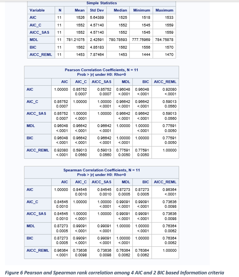
AIC = -2 log L + 2(p+k+1)
AICC= -2 log L + [2(p+k+1) (n/(n-p-k-2))]
Where,
p = number of fixed effect terms
k = number of random effect terms
n = total sample size for random effect model and number of subjects in case of repeated measures
* In large sample AIC and AICC are nearly equivalent
ΔAICC = AICCi- AICC min Best candidate models = (ΔAICC <=2)
AICCsas = AICC reported by SAS PROC Mixed using ML
AICCREML = AICC reported by SAS PROC Mixed using REML
MDL =1/2 {-2 log L + [log(n) (p+k+1)]} (Hoeting et. al 2006)
Δ MDL = MDLi- MDL min Best candidate models = (Δ MDL <=1)
In the ALLMIXED macro, the best candidate model’s selection criterion based on Δ MDL is <=1. This new criterion is comparable to the criterion used for Δ AICC (<=2)
BIC = -2 log L + [log(n) (p+k+1)] (SAS Institute 2006)
Penalty factor % = (pf i / -2 log L ref) *100
AICC weights =Exp(-0.5*Delta AICC i) / Sum of (Exp(-0.5*Delta AICC i) ) all best candidate model
MDL weights =Exp(-0.5*Delta MDL i) / Sum of (Exp(-0.5*Delta MDL i) ) all best candidate model
AICC weight ratio = AICC weight / Max (AICC weight)
MDL weight ratio = MDL weight / Max (MDL weight)
Step 3 in all possible mixed model fixed effect selection
All combination of models associated with the user-specified fixed effects subset range (start:2 and stop: 3) are generated by the ALLMIXED macro and their information criteria statistics, AICC and MDL are
compared in this step. Users can optionally specify certain fixed effects as “MUST HAVE” and other fixed effects as “SELECTABLE” in all possible model selection. All combination of mixed model using the fixed
effects listed in “SELECTABLE” category are generated in this step and the following statistics are estimated.
- Variance inflation statistics (VIF) for each continuous predictor variables in the model.
- PRESS and SSE for each model considered. Big differences between PRESS and SSE are an indication of significance outliers in the model
- Information criteria estimates based on REML: AICCreml
- Information criteria estimates based on ML: AIC, AICC, AICCsas, MDL, and BIC.
-------------------------------------------------------------------------------------------------------------------------------------------------------------------------------------------------------------------
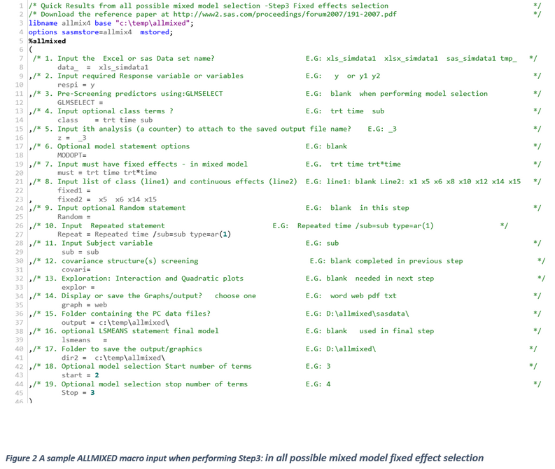
ALLMIXED SAS macro help – Step 3 Repeated measure covariance type selection
- Input the Excel file name or SAS data set name?
Descriptions and Explanation: Include the data type name (XLS, TAB, TXT, SAS, TMP) and name of the data set on which you would like to perform pre-screening.
Options / Examples:
- xls_SIMDATA1: Data type is EXCEL, and the file name is SIMDATA1. Make sure to include the separator character '_'.
SAS_SIMDATA1: Data type is permanent SAS (SD7SAS) and the SAS permanent data name is SIMDATA1
TMP_SIMDATA1: Data type is temporary SAS data and file name is SIMDATA1.
- Input required Response variable or variables
Descriptions and Explanation: Input the continuous response (dependent) variable name (or names). The name should match the variable names in the data. You can include multiple responses
Options / Examples:
- Y Y1 Y2
- Pre-screening fixed variables using GLMSELECT
Descriptions and Explanation: This field should be left blank in the fixed effects selection.
Options / Examples:
- GLMSELECT=
- Input optional CLASS terms
Descriptions and Explanation: Input the names of the categorical variables that will be included in the CLASS statement in PROC Mixed.
Options / Examples:
Class= TRT time sub
- Input ith analysis (a counter) to attach to the saved output file name
Descriptions and Explanation: Input any numeric and categorical character to track the number of the analysis that you are running using this data. For example, if you input 1A, the output file created in this step would be called SIMDATA11A.ext.
Options / Examples:
Z = -1
Z = 1A
- Input “MUST-HAVE” fixed effects in Mixed model
Descriptions and Explanation: Input the “MUST_HAVE” fixed effect model terms that you must include in the MODEL statement.
Options / Examples:
TRT TIME TRT*TIME
- Input the list of model terms used in ALL possible Fixed effect selection
Descriptions and Explanation: Input the list of model terms that will be used in all possible model selection. (DO NOT USE X1-X15 syntax.) Input all categorical variables terms in the first line of input. Input all continuous terms in the second line. VIF statistics will be computed for these predictors.
Input any other predictors and model terms in the second line of input.
Options / Examples:
C1 c2 c3 ----------> first line
x5, x14, x15, X6----------> second line
- Fixed1 =
- Fixed2 = x5 x6 x14 x15
- Input Optional Random statement(s)
Descriptions and Explanation: Input PROC MIXED RANDOM statements.
Options / Examples:
- Random= Random INT /sub=sub
- Random =
- Input Repeated Statement
Descriptions and Explanation: Input PROC MIXED REPEATED statement including the selected covariance.
Options / Examples:
- Repeat = Repeated time / sub=sub type=AR(1)
- Input the subject variable name
Descriptions and Explanation: In case of repeated measures data, input the subject variable name. This forces the pre-screening to do initial selection at the subject level.
Options / Examples:
- Id, subject, or blank
Sub = Sub
- covariance structure(s) screening
Descriptions and Explanation: This field should be left blank for all possible subset selection.
- Display or save the Graphs/output? choose one
Descriptions and Explanation: Option for viewing and saving all output files in a folder specified in input number 17.
WORD: Output and all SAS graphics are saved together in the user-specified folder as a single RTF format.
WEB: Output and graphics are saved in the user-specified folder as a single HTML file.
PDF: Output and graphics are saved in the user-specified folder and as a single PDF file.
TXT: Output is saved as a TXT file in all SAS versions. No output is displayed in the OUTPUT window. All graphic files are saved as PNG format in the user-specified folder.
- Folder containing the PC data files
Descriptions and Explanation: Input the full path of the folder containing the source data file.
Options / Examples:
- 😧\allmixed\sasdata\ - folder name SASDATA on drive D
Make sure that you include the backslash (\) at the end of the folder name.
OUTPUT= c:\temp\allmixed\
- Folder to save the output/graphics?
Descriptions and Explanation: To save the SAS graphics, data, and output files, input the output folder name. If the 14 field is left blank, the output files are saved in the default folder.
Options / Examples:
Dir2= C:\temp\allmixed\
- Input optional Start subset- all possible subset selection
Descriptions and Explanation: Input the number of all possible subsets to begin all possible subset selection.
Options / Examples:
- 2 – Start all possible subset selection search starting from subset 2.
- 1 – Start the all possible subset selection search starting from subset 1.
- Start = 2
- Input optional stop subset- all possible subset selection
Descriptions and Explanation: Input the number of all possible subsets to stop.
Options / Examples:
- 8 – Stop all possible subset selection search from subset 8.
- 7 – Stop all possible subset selection search from subset 7.
- Stop = 3
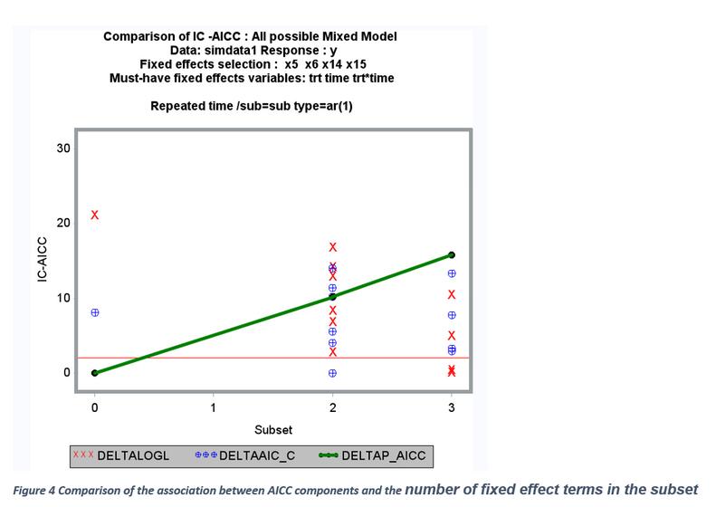
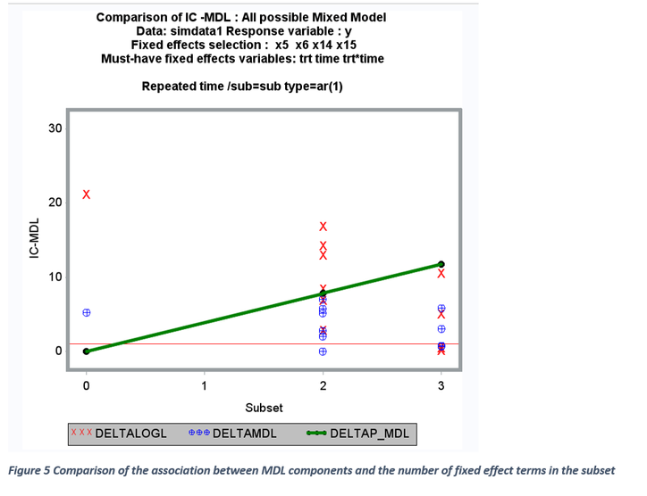
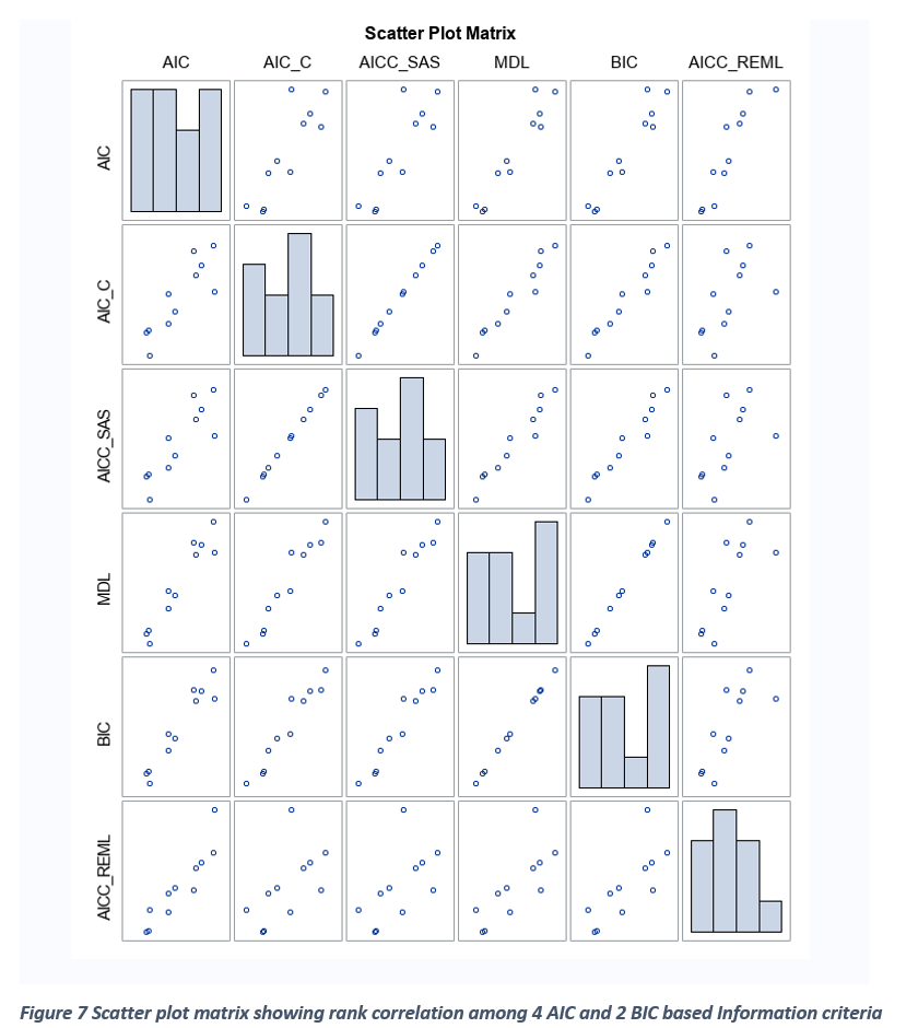
All IC statistics reported here are made out of two components: a) Log likelihood estimate (-2 log L ) b) penalty factor (pf). For a given model, -2 log L value is constant and influenced by degree of model fit, variable included and not included in the model, presence of influential outliers, and model specification errors. The penalty factor is made from number of fixed (p) and random effects (k) and the sample size (n). When all possible model selection involving only the fixed effects are carried out, the sample size and the number of random effects become constant. Therefore, only the number of fixed factors becomes the determining component of the penalty factor. The relationship between penalty factor and the number of fixed effects between AIC_C, AICCreml, and MDL are shown in Figures 4 and 5. The penalty factor for the AICCreml becomes constant because this penalty factor does not include any fixed effects and only the number of random effects (which is a constant) is included. The penalty factors for AICC and MDL shows a positive linear effect associated with the increase in the number of fixed effects. Thus, the degree of overall penalty is usually stronger for MDL than the AICC initially and declined slowly and this clear in the ratio between MDL penalty % and AICC penalty and the relationship is clearly shown in Figure 5. The components of AICC and MDL ( -2 log l and the penalty factor) are graphically compared in Figure 7. For a given model, -2log L value is constant when estimating AICC and MDL and it decreases linearly with an increase in the number of fixed terms. But, within a subset (two, and three variable subset), the -2 log L value varies a lot whereas all the models within a subset have the same penalty factor for both AICC and MDL (Figure 4 and 5). Also, delta AICC statistic favors parsimonious model (2) whereas MDL statistic favors models with large number of model terms (2 and 3subsets) especially in a small data set (50 subjects in repeated measures data) (Figures 10 and 11).
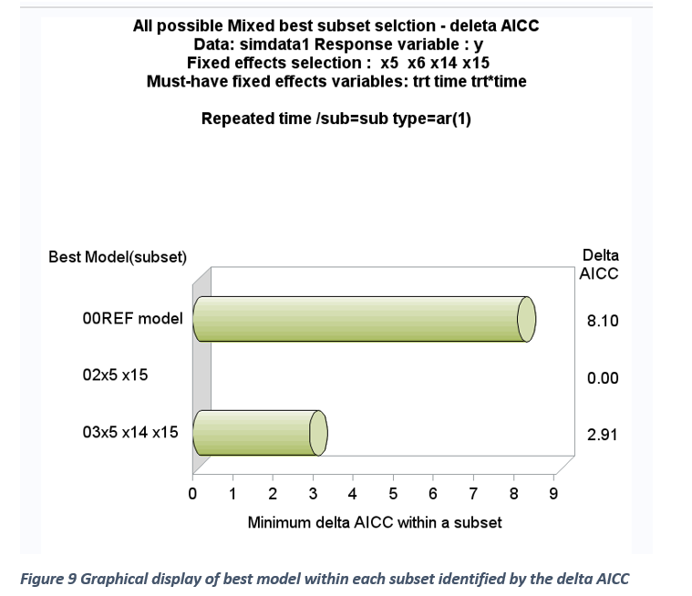
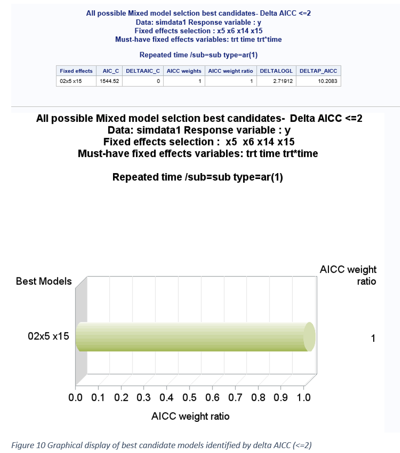
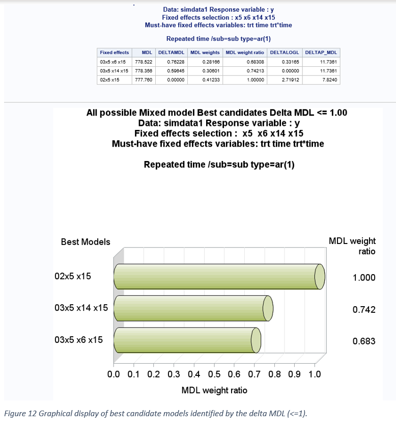
Graphical display of best models within each subset based on smallest ΔAICC and ΔMDL within each subset are shown in Figures 9-12. The 2-variable subset was identified as the best subset based on AICC and MDL. Graphical display of overall best candidate models based on ΔAICC <= 2 and ΔMDL <=1 is shown in Figures 10 and 12. The model weight ratios are compared between the selected best candidates’ models. The true two variable fixed effect models (X5 and X15) were selected among the best candidates’ models based on both AICC and MDL. The model selection results for this simulated large data (50 subjects, 5 repeated measures) clearly shows that ΔAICC favors parsimonious model whereas ΔMDL favors overestimated model. However, when the total sample size is very large (250), ΔMDL favors more parsimonious model than AICC.GRAPHICAL EXPLORATION FOR MULTICOLLINARITY AND INFLUENTIAL OUTLIERS
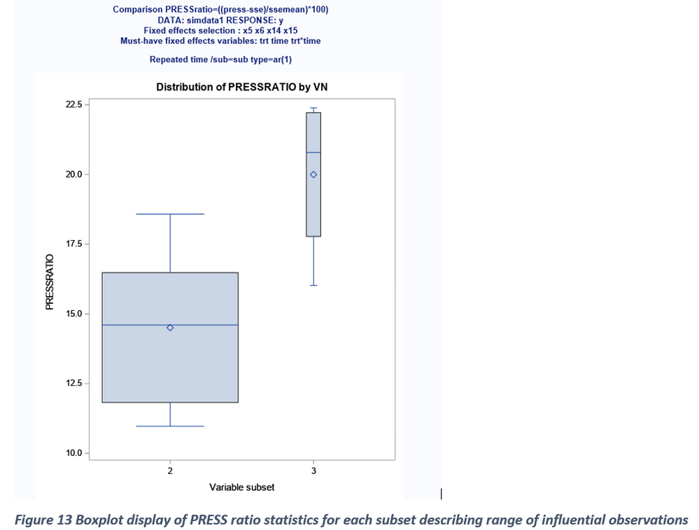
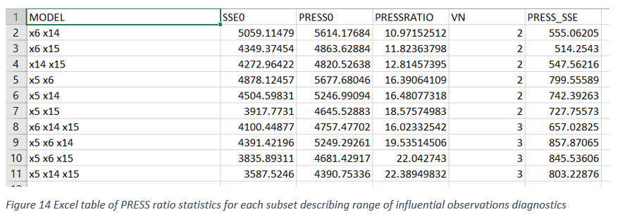
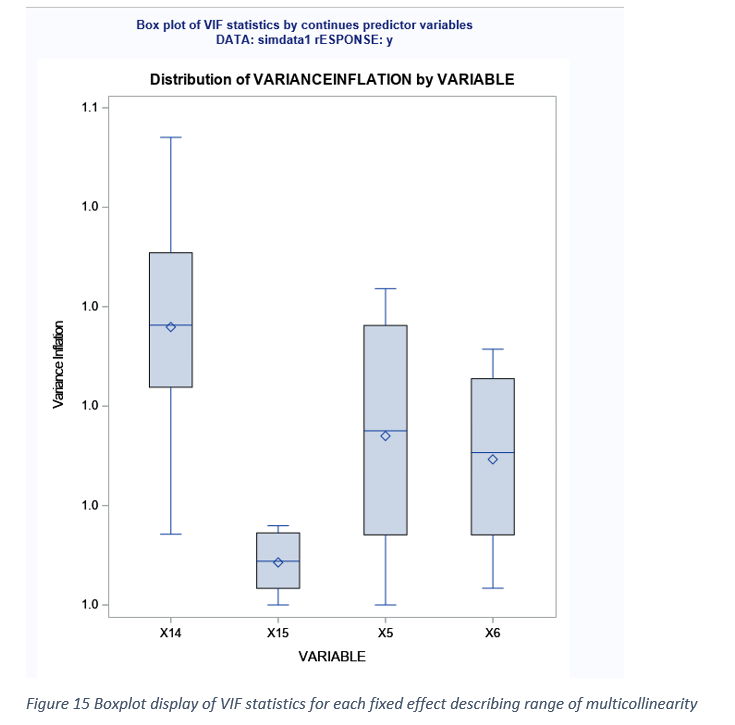
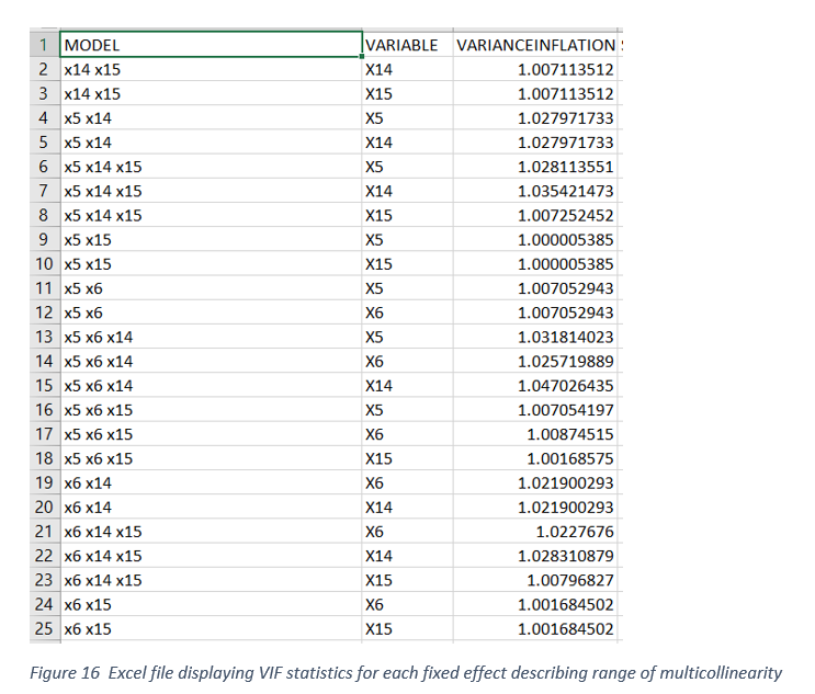
Differences between PRESS and SSE can be assessed by the magnitude of differences or the ratio estimates. Big differences between PRESS and SSE can be attributed to the presence of influential outliers in all possible models evaluated (Figure 13-14). Severe multicollinearity (Variance inflation factor > 10) among predictor variables in mixed model analysis can result in unstable parameter estimates with inflated standard errors. When a fixed effect predictor involved in a collinear relationship is dropped from the model, the sign and size of the remaining predictor variable estimates can change dramatically. Therefore, presence of high degree of multicollinearity can impact fixed effect selection. Therefore, assessing the degree of multicollinearity for each of the continuous fixed effects in all possible model selection can help to select the best model from the set of best candidate models. Variable(s) not contributing multicollinearity could be preferred over the variables significantly contributing to multicollinearity. Figure 15 shows the box-plot display of VIF distribution for all the continuous predictors included in model selection. Because the data used in the study are simulated from known properties multicollinearity should not exists and it is clearly shown in Figure15 where VIF values were less than 2 for all the predictor variables.
Reference
Fernandez, G. (2007) Model Selection in PROC MIXED - A User-friendly SAS® Macro Application SAS Global Forum proceedings 191-2007
https://support.sas.com/resources/papers/proceedings/proceedings/forum2007/191-2007.pdf
Hoeting, J.A, Davis R.A Merton A.A and Thompson S. E (2006) Model selection for Geostatistical Models Ecological Applications, 16(1), pp. 87–98
- Mark as Read
- Mark as New
- Bookmark
- Permalink
- Report Inappropriate Content
After testing with the following dataset, it was revealed that the compiled ALLmix macro was hard coded to use a fixed variable in the input data set, which is the variable 'time'.
Because my testing data set does not have the 'time' variable, the macro failed to run.
I strongly suggest the author open the source of the compiled macro. Otherwise, it is hard for others to use it and nobody will use it in the future, though the author has contributed a lot of time to write the program!
In addition, the compiled macro only works under Windows SAS but not Linux SAS. For SAS OnDemand for Academics, due to its Linux SAS, the compiled macro can not run.
This is my testing codes:
libname allmix4 "C:\Users\cheng\Downloads\ALLmixed";
%let wd=C:\Users\cheng\Downloads\ALLmixed\;
options sasmstore=allmix4 mstored;
/*Generate data for testing*/
*https://facweb.cdm.depaul.edu/sjost/csc423/documents/glmselect-summary.pdf;
data analysisData testData;
drop i j;
array x{20} x1-x20;
do i=1 to 5000;
/* Continuous predictors */
do j=1 to 20;
x{j} = ranuni(1);
end;
/* Classification variables */
c1 = int(1.5+ranuni(1)*7);
c2 = 1 + mod(i,3);
c3 = int(ranuni(1)*15);
yTrue = 2 + 5*x17- 8*x5 + 7*x9*c2- 7*x1*x2 + 6*(c1=2) + 5*(c1=5);
y= yTrue + 6*rannor(1);
if ranuni(1) < 2/3 then output analysisData;
else output testData;
end;
run;
proc datasets nolist;
copy in=work out=Allmix4 move;
select analysisData;
run;
%allmixed
(
/* 1. Input the Excel or sas Data set name? E.G: xls_simdata1 xlsx_simdata1 sas_simdata1 tmp_ */
data_ = sas_analysisdata
,/* 2. Input required Response variable or variables E.G: y or y1 y2 */
respi = y
,/* 3. Pre-Screening predictors using:GLMSELECT E.G: blank when performing model selection */
GLMSELECT =
,/* 4. Input optional class terms ? E.G: trt time sub */
class = c1 c2 c3
,/* 5. Input ith analysis (a counter) to attach to the saved output file name? E.G: _3 */
z = _3
,/* 6. Optional model statement options E.G: blank */
MODOPT=
,/* 7. Input must have fixed effects - in mixed model E.G. trt time trt*time */
must = x1 x2 x5 x10 x13 x9 x17 c1 c2 c3 x1*c1 x2*c2
,/* 8. Input list of class (line1) and continuous effects (line2) E.G: line1: blank Line2: x1 x5 x6 x8 x10 x12 x14 x15 */
fixed1 = c1 c2 c3
, fixed2 = x1 x2 x5 x10 x9 x13 x17
,/* 9. Input optional Random statement E.G: blank in this step */
Random =
,/* 10. Input Repeated statement E.G: Repeated time /sub=sub type=ar(1) */
Repeat = Repeated time /sub=sub type=ar(1)
,/* 11. Input Subject variable E.G: sub */
sub =
,/* 12. covariance structure(s) screening E.G: blank completed in previous step */
covari=
,/* 13. Exploration: Interaction and Quadratic plots E.G. blank needed in next step */
explor =
,/* 14. Display or save the Graphs/output? choose one E.G: word web pdf txt */
graph = web
,/* 15. Folder containing the PC data files? E.G: D:\allmixed\sasdata\ */
output = &wd
,/* 16. optional LSMEANS statement final model E.G: blank used in final step */
lsmeans =
,/* 17. Folder to save the output/graphics E.G: D:\allmixed\ */
dir2 = &wd
,/* 18. Optional model selection Start number of terms E.G: 3 */
start = 2
,/* 19. Optional model selection stop number of terms E.G: 4 */
Stop = 3
)
- Mark as Read
- Mark as New
- Bookmark
- Permalink
- Report Inappropriate Content
After further evaluation of the macro, it reveals that 'Repeat = Repeated time /sub=sub type=ar(1)' needs to be replaced with blank, as the input dataset does not contain the time variable. So the macro can run successfully in Windows system.
- Mark as Read
- Mark as New
- Bookmark
- Permalink
- Report Inappropriate Content
I found your compiled SAS macro allmix4 is very helpful for modeling. However, I can only run it successfully in SAS 9.4 Workbench in Windows.
As SAS OnDemand for Academics is free, I would like to use your macro in the cloud computing system that is based on Linux system. After evaluating your allmix4 macro in SAS OnDemand for Academics, I found the following error:
SAS AI and Machine Learning Courses
The rapid growth of AI technologies is driving an AI skills gap and demand for AI talent. Ready to grow your AI literacy? SAS offers free ways to get started for beginners, business leaders, and analytics professionals of all skill levels. Your future self will thank you.

