- Home
- /
- SAS Communities Library
- /
- Tip: How to Derive New Variables for Better Predictive Models
- RSS Feed
- Mark as New
- Mark as Read
- Bookmark
- Subscribe
- Printer Friendly Page
- Report Inappropriate Content
Tip: How to Derive New Variables for Better Predictive Models
- Article History
- RSS Feed
- Mark as New
- Mark as Read
- Bookmark
- Subscribe
- Printer Friendly Page
- Report Inappropriate Content
Introduction
There are many important components in making data mining work for you. One of the most important parts is ensuring that you glean all of the information you can from your data. Sometimes simple transformations and replacements can make a big impact on your model. The SAS® Enterprise Miner™ nodes make it easy to make these types of changes. Let’s explore the topic now.
Data
Here we are using Titanic data. This data set contains 891 observations and 12 variables.
Variable Descriptions:
Survival Survival (0 = No; 1 = Yes)
Pclass Passenger Class (1 = 1st, 2 = 2nd , 3 = 3rd )
Name Name
Sex Sex
Age Age
Sibsp Number of Siblings/ Spouses Aboard
Parch Number of Parents/Children Aboard
Ticket Ticket Number
Fare Passenger Fare
Cabin Cabin
Embarked Port of Embarkation (C = Cherbourg, Q = Queenstown, S = Southamton)
We will build a model where we have to predict the fate of the passengers aboard the RMS Titanic, which sank in the North Atlantic Ocean in the early morning of April 15, 1912, after colliding with an iceberg.
According to Wikipedia, a disproportionate number of men were left aboard because a “women and children first” protocol was followed when loading lifeboats. There were not enough lifeboats to accommodate all of those aboard, only a fraction of the passengers survived.
Our first model without any data modifications
We can build a simple model using a Decision Tree as shown below using variables given in the Titanic data. Since the name, cabin number and ticket number are all unique to each passenger; let’s reject those variables for now. We will use all other variables as predictors to build this model.
Run the flow and check the Tree results. We will use misclassification rate as the measure of the best model. Notice that the Misclassification Rate for this model is 0.17284 as shown below.
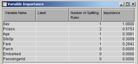
Check the Variable Importance table in the Tree results. Notice that Sex, Pclass, Age, SibSp and Fare are important variables.
Our first model with data modifications
How can we get a better model? Here we can create new variables from the available variables to get more value from them.
While the ticket, cabin and name data isn’t useful since they were unique to each passenger; maybe a substring of those text strings could be useful to build a new predictor. We can start with the name field. If we explore a passenger’s name we see the following:
Moran, Mr. James
A passenger’s title can reflect gender, position on the ship (doctors, officer & wealthy people), and access to lifeboats (where “Master” superseded “Mr”). Perhaps the passenger’s title might give us a little more insight.
If we explore the dataset we see many titles including Mr, Mrs, Miss, Master, Lady and the Countess. The title ‘Master’ was used for unmarried boys. We have very few of the following titles: Captain, Don, Major and Sir. All of these are either military titles, or rich people. We might be able to create a new variable which can be an important predictor other than age, gender, etc.
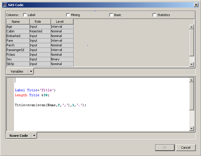
In order to extract these titles to make new variables, we can use the Transform node. We can use the SAS Code window in the Transform node to create a new variable called “Title”.
Add a Transform Variables node between the IDS node and the Tree node as shown below.
Select Transform Variables node, open SAS Code editor and enter code mentioned below. Here, we have used the SCAN function to extract the title from the character variable Name.
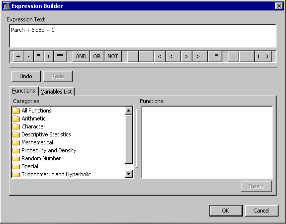
What else can we do to get more information from existing variables? There are two variables SibSb and Parch that indicate the number of family members each passenger is travelling with. We can assume that a large family might have trouble gathering all family members as they all try to get off the sinking ship, so we try to combine the two variables into a new one, FamilySize. Again we can use the Transform node to create a new variable.
We can use either the SAS Code editor or the Formula Builder to create this variable. Let’s use the Formula Builder.
- Select the Transform node and open the Formulas window.
- Select the “Create” button.
- In the “Edit Transformation” window, enter “FamilySize” in the Name field to create a variable called “FamilySize”.
- Select the “Build” button. Create the following formula in the Expression Builder. We just add the number of siblings, spouses, parents and children the passenger had with them, and plus one for their own existence of course.
5. Select “OK” and save your changes.
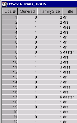
6. Run the flow from the Transform node and check the exported data. Explore the new variables “Title” and “FamilySize”.
Run the flow and check the Tree results. Notice that this model performed better than the previous model. The Misclassification Rate for this model is 0.160494 as shown below.
Check the Variable Importance table in the Tree results. Notice that Title, FamilySize, Pclass, Age and Sex are important variables and are used in a tree to build the model. You can see that new variables Title and FamilySize have higher importance than SibSp and Fare.
Our next model with data modifications
What else we can do to improve this model? If you look at all observations of the Title variable, you will notice that there are a few very rare titles that won’t give our model much information to work with, so let’s combine a few of the most unusual titles. For the ladies, we have “Lady”, “the Countess”, “Dana”, “Mme”, “Mlle” and “Johkheer”. All of these are rich ladies traveling in first class. We can combine these separate groups into the “Lady” group.
For the men, we have a handful of titles: Captain, Don, Major and Sir. All of these are either military titles, or rich people. We can combine these titles into the “Sir” group.
We can use the Replacement node to reduce the number of levels. Add a Replacement node between the Transform node and the Tree node as shown below.
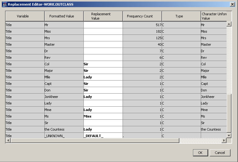
Select the Replacement node and open the Replacement Editor for class variables. As explained above, combine a few of the unusual titles into a single category as shown below. Replace “Col”, “Major”, “Capt” and “Don” with “Sir” and “Jonkheer”, “Mme”, “Mlle” and “the Countess” with “Lady”. Replace “Ms” with “Miss”. Save your changes.
Run the flow and check the Tree results. Notice that this model performed better than the previous model. Notice that the Misclassification Rate for this model is 0.150393 as shown below.
Comparing models with and without data manipulation
You can use the Model Comparison node to compare all three models.
Check the Model Comparison results. Notice that Tree_Model3 was selected as the best model using the misclassification rate as the metric for model selection.
Summary
This example shows that a little bit of effort in transforming your data can go a long way toward improving your model. With just a few transformations we’ve begun to see an improvement in classification accuracy. Imagine the improvements you might achieve with a bit more effort.
- Mark as Read
- Mark as New
- Bookmark
- Permalink
- Report Inappropriate Content
Nice example. Simple enough to understand with real misclassification improvement. I have printed it and will keep it in my notebook to remind me to try these types of enhancements. Thank you!
- Mark as Read
- Mark as New
- Bookmark
- Permalink
- Report Inappropriate Content
I am glad you find this tip useful, Toptoad713! I personally find the titanic example fascinating. This is a great learning problem because the data set is relatively simple, with some missing values thrown in, and just enough noise to make things interesting.
- Mark as Read
- Mark as New
- Bookmark
- Permalink
- Report Inappropriate Content
Is there a real dataset that I could work upon....Thanks
- Mark as Read
- Mark as New
- Bookmark
- Permalink
- Report Inappropriate Content
, Here is a repository with real data sets (UCI Machine Learning Repository: Data Sets). Plot your target with some of their inputs and then try to capture that relation with a variable transformation. Try the transformations in these examples, as well as the ones described in the help for the Transform Variables node. The section "Best Power Transformations" is really useful... Not 100% sure, but I think this is a real data set. Good luck! -Miguel
- Mark as Read
- Mark as New
- Bookmark
- Permalink
- Report Inappropriate Content
Thank you Miguel, appreciate it.
- Mark as Read
- Mark as New
- Bookmark
- Permalink
- Report Inappropriate Content
Miguel, thank you for providing information about real data sets repository and Transform Variables help document. Sanjiv, for your reference, I have attached the data set I used in this example. Thank you!
- Mark as Read
- Mark as New
- Bookmark
- Permalink
- Report Inappropriate Content
That's great...Thank you.
April 27 – 30 | Gaylord Texan | Grapevine, Texas
Registration is open
Walk in ready to learn. Walk out ready to deliver. This is the data and AI conference you can't afford to miss.
Register now and save with the early bird rate—just $795!
SAS AI and Machine Learning Courses
The rapid growth of AI technologies is driving an AI skills gap and demand for AI talent. Ready to grow your AI literacy? SAS offers free ways to get started for beginners, business leaders, and analytics professionals of all skill levels. Your future self will thank you.
- Find more articles tagged with:
- tips&tricks


