- Home
- /
- SAS Communities Library
- /
- Tip: Getting started with Time Series Clustering
- RSS Feed
- Mark as New
- Mark as Read
- Bookmark
- Subscribe
- Printer Friendly Page
- Report Inappropriate Content
Tip: Getting started with Time Series Clustering
- Article History
- RSS Feed
- Mark as New
- Mark as Read
- Bookmark
- Subscribe
- Printer Friendly Page
- Report Inappropriate Content
When you work with data measured over time, it is sometimes useful to group the time series. Time Series Clustering (TSC) can be used to find stocks that behave in a similar way, products with similar sales cycles, or regions with similar temperature profiles.
TSC can also help you incorporate time series in traditional data mining applications such as customer churn prediction and fraud identification. For example, suppose you have a hunch that customer’s behavior over time would help predict churn or fraud. How would you incorporate the temporal pattern as a predictor in your model, where the unit of analysis is the customer? You can achieve this by categorizing each of the original series and using the category labels as inputs in your predictive model:
Of course you could eyeball the series’ shapes and categorize them manually into, say, flat series, shifty series, trending series, and so on. But that would be tedious, if not impractical, if you have more than a few series. This tip shows how to automate series labeling using clustering techniques in SAS® Enterprise Miner™.
Data
The data for this tip are 2008 individual mortality data from Mexico (Wickham, 2014). The dataset includes the following variables:
- cod = Cause of death code
- disease = corresponding disease. There are 1194 diseases in total.
- hod = Hour of day
- Mortality - frequency (freq) and proportion (prop) of deaths at each time point
The raw dataset consists of time profiles for 1194 diseases, stacked one on top of the other:
Here is a plot of the time profile for the first disease, Acute Bronchitis:
SAS Enterprise Miner flow
This simple process flow prepares the mortality data for time series analysis, then clusters the diseases based on their time profiles.
Input Data Source Node (HOD2)
I defined variable metadata as follows:
- Time ID: hour of day
- Target: proportion of death
- Cross ID: Disease
SAS Code Node
I used SAS code to filter rare diseases. 214 diseases remained after filtering.
TS Data Preparation Node
This node transforms the input data to a proper time series format for similarity analysis. In the transposed dataset, each disease profile time series becomes an input variable. I set node properties as follows:
- (Time Interval) Specify an Interval: Automatic (This is the default)
- (Transpose Options): Transpose: Yes.
This is a snippet of the exported data:
Transposed Time Series (Partial)
Notice that we now have a time series dataset: the rows represent ordered, equally spaced time points; there is one column per disease; and the values are proportion of deaths for a given disease at a given time of day.
TS Similarity Node
I used the following node properties:
- (Clustering Options) Number of Clusters: 5.
- Output Data Set: Clustering segment
The node first creates a similarity matrix, a representation of the similarity/distance of each pair of individual series. Then it uses hierarchical clustering to group similar diseases. After some initial exploration, I settled on a 5-cluster solution.
The node produces familiar clustering output such as a constellation plot and dendrogram. But in addition to the graphical output, the node reports the cluster assignment for each series. I merged this series-to-cluster map to my raw input data for the plots below.
Results
Before drilling into the clusters, let’s examine some of the elements in the similarity matrix computed by the TS Similarity node. I created all of the plots with SAS and Proc SGPANEL.
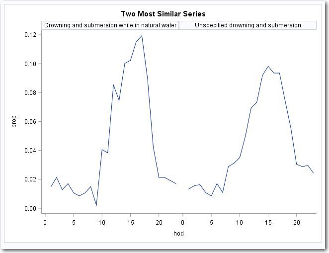
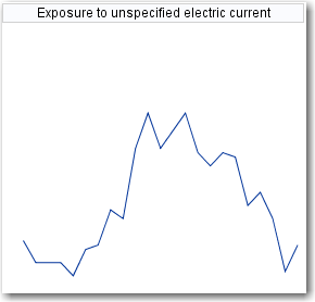
Here are the two pairs (diseases) with the greatest similarity (i.e., the smallest sum of squared difference across time points).
Most similar series
Both series represent types of drowning. Since they have greatest similarity among any pair of diseases, these are the first two series joined by the hierarchical clustering algorithm.
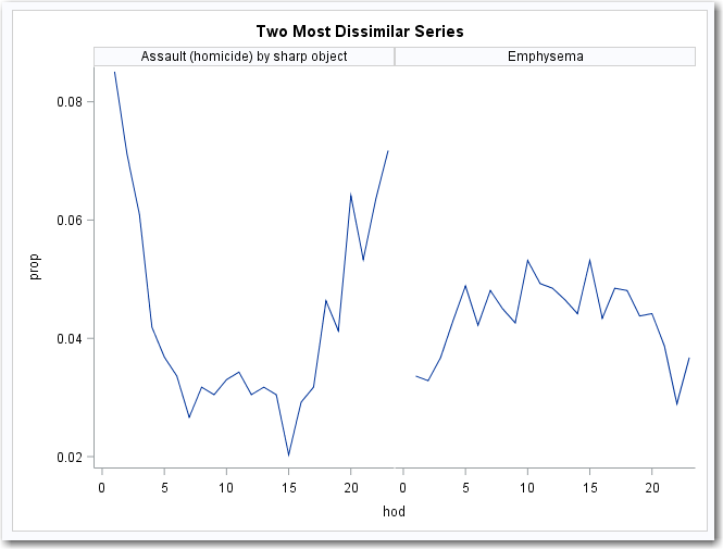
For comparison, here are the two most dissimilar series (i.e., diseases with the largest sum of squared differences across time):
Most dissimilar series
Visually, these series are certainly easy to distinguish. One is U-shaped, with big variation over time. The other is flatter with an inverted U-shape.
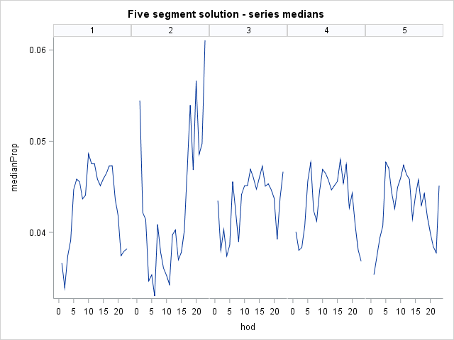
To explore the five clusters, I plotted the overall time profile by cluster (in TSC, these time profiles represent the cluster centers):
Cluster Centers
Here Cluster 2 stands out, not only because mortality varied greatly with time compared to the other clusters, but also because it was the only cluster with a U-shaped pattern. In other words, Cluster 2 seems to represent deaths that spike late at night into the early morning, and rarely occur during the day.
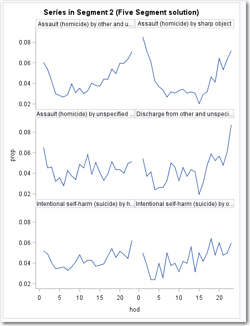
Drilling into Cluster 2, here are the first six diseases in the cluster:
In general, these diseases reflect the aforementioned U pattern, with high incidence at night. Homicides and suicides dominate this cluster.
In contrast, series in cluster 1 tend to have an inverted U pattern: they occur primarily during daytime hours (drownings, electrocutions) or in the early morning (SIDS).
Conclusion
As you can see, getting started with Time Series Clustering is easy with SAS Enterprise Miner. If the ultimate goal were a predictive model, such as a model to predict the economic impact of each, we could now use the derived clusters as inputs.
Because the TS Similarity node gives you the option to export a distance matrix, you can use any EM clustering node for clustering time series. Just choose the Output Data Set: Distance Matrix option in node properties before running the TS Similarity node. I obtained the distance matrix the same way for two of the above plots.
The TS Similarity node can also be used to identify series that are similar to a target/reference series. For example, to identify financial behavior that is similar to known abusive or fraudulent behavior. While not an issue with the mortality data used in this tip, the node can also handle series of varying lengths via time warping.
Further Reading
For more about the mortality data used in this tip, see:
Wickham, H. (2014). Tidy Data. Journal of Statistical Software, Vol 59.
And here is a great resource on Time Series Data Mining in SAS Enterprise Miner:
https://support.sas.com/resources/papers/proceedings11/160-2011.pdf
- Mark as Read
- Mark as New
- Bookmark
- Permalink
- Report Inappropriate Content
Hi @rayIII! Thanks for an intriguing article - this has certainly put my brain into overdrive 🙂 I don't have access to Enterprise Miner but would still like to use this type of analysis. Do you know of any papers or SAS Documentation that talks about using Base SAS? I have searched and unable to find anything; I've got a number of theoretical articles, which I'm so far OK understanding but would like something more SAS-specific. I assume it's more complicated that using PROC TIMEDATA and then PROC CLUSTER 😉
Thanks so much and if you're going to be at SGF, would love to talk face-to-face about this.
Have a great day
Chris
- Mark as Read
- Mark as New
- Bookmark
- Permalink
- Report Inappropriate Content
Hi, Chris. Great--I'm glad you found it useful. If you don't have access to EM, you could start exploring TSC with PROC SIMILARITY and PROC CLUSTER. (PROC SIMILARITY requires ETS, but unlike PROC DISTANCE, is designed specifically for dealing with time series.)
I'm glad you mentioned reading some articles because TSC is a big topic--there are lots of different distance metrics and clustering approaches (e.g., clustering of shapes vs. clustering of structures). Plotting the clustered series with your favorite SAS graphing tools will help make sure you are on the right path.
Good luck!
Ray
April 27 – 30 | Gaylord Texan | Grapevine, Texas
Registration is open
Walk in ready to learn. Walk out ready to deliver. This is the data and AI conference you can't afford to miss.
Register now and save with the early bird rate—just $795!
SAS AI and Machine Learning Courses
The rapid growth of AI technologies is driving an AI skills gap and demand for AI talent. Ready to grow your AI literacy? SAS offers free ways to get started for beginners, business leaders, and analytics professionals of all skill levels. Your future self will thank you.
- Find more articles tagged with:
- Cluster Analysis
- clustering
- data mining
- Time Series


