- Home
- /
- SAS Communities Library
- /
- SAS Forecasting Tools: Powerfully Predicting the Future
- RSS Feed
- Mark as New
- Mark as Read
- Bookmark
- Subscribe
- Printer Friendly Page
- Report Inappropriate Content
SAS Forecasting Tools: Powerfully Predicting the Future
- Article History
- RSS Feed
- Mark as New
- Mark as Read
- Bookmark
- Subscribe
- Printer Friendly Page
- Report Inappropriate Content
CONCEPTUAL OVERVIEW OF FORECASTING Forecasting differs from other predictive analytics. Ordinary predictive analytics simply predict an outcome from inputs, whereas forecasting is done using time series data. To conduct forecasting, you must have data over a historic time period with a time variable in the data set. It is essential that you use appropriate methods when working with time series data. SAS forecasting tools let you do this easily.

- how many kids are in his class
- how many girls are in his class
- how many kids have Frozen-themed attire
- what day of the week Valentine’s Day lands on
Note that there is no time component. The four inputs listed are the independent variables and the number of Frozen Valentine’s cards he gets is the dependent variable (output).
Forecasting Example But let’s imagine that a time component is introduced. One variable might be how many cards Finn got each year for the last five years. Another variable might be how many cards were exchanged in Ms. Schmidt’s class over the last five years (input variable over time). Now we have a very simple forecasting example.
Cycles and Trends Time series data often exhibit cycles and trends. Cycles may be:
- daily (e.g., air temperature may peak in the afternoon every day)
- weekly (e.g., shoe sales may peak weekly on Saturdays)
- seasonally (e.g., natural gas usage may peak in winter) …and so on…
Below is US electricity production from 2001-2013 graphed in SAS Forecast Server and forecasted for 2014. The dots are the data, and the line is the model. We see a clear seasonal pattern, with a high peak in summer, and a lower peak in winter. This seasonality is also expressed in the forecast for 2014.
Trends show a long-term increase or decrease. For example, we may see electricity generation increasing over a long period of time. A trend may be modeled as a deterministic mathematical function, such as a polynomial, logarithm or exponential function (of time).
Looking at the same electricity generation graph, we can see that from 2001 to 2008 there appears to be an upward linear trend, during that truncated time period. Cycles and trends can co-occur; they are not mutually exclusive.
Serial Correlation
Once a time variable is introduced, predictive analytical methods such as least squares regression are no longer valid, because neither the observations nor the errors are independent, they are serially correlated. For example, today’s air temperature is correlated to yesterday’s air temperature. Some folks try to use regression for time series data. SAD! We must employ special time series analytical techniques. Examples include:
- ARIMA – Autoregressive Integrated Moving Average models, also called Box-Jenkins models
- Exponential Smoothing Models
- UCM – Unexplained Components Models
Let’s take ARIMA as an example. To address the issue of serial correlation, ARIMA introduces lagged terms. In flexible programming tools like ETS, you select your own p (autoregressive term), d (difference term), and q (moving average term). Autoregressive terms are essentially lags on the observed values, and moving average terms are lags on the errors. To determine your pdq’s, you can use diagnostic graphs like the Partial AutoCorrelation Function (PACF) to determine an appropriate AR (p) lag and the Inverse Autocorrelation Function (IACF) to determine an appropriate MA (q) lag. Or you can use a super groovy automated tool like Forecast Server, which will select the best models using these diagnostics for you.
You can think of an ARIMA as a model that tries to separate the signal from the noise, and then extrapolates that signal into the future. A random walk is the simplest ARIMA (0,1,0), i.e., p=0, d=1, and q=0.
FORECASTING IN SAS PRODUCTS
Forecasting is available in a number of SAS products. If you wish to develop your own models and select your own pdq, SAS/ETS or SAS Econometrics is a good way to go. If you prefer to let the software intelligently select the best pdq pretty darn quickly, then Forecast Server or SAS Visual Forecasting is a better route. If you are just beginning to dabble in forecasting, and don’t have any background in statistics or time series analyses, I recommend Visual Analytics as the best way to dip your toe into the forecasting world.
If you are working with a customer who is changing software, or using more than one SAS product, be aware that they may get different results. For example, Visual Analytics forecasting results differ from Forecast Server results. As I have mentioned in other blogs, in order to replicate results as closely as possible, it is important that you know what defaults or options were used versus what defaults or options you are using with a newer or different SAS software product.
Visual Analytics 7.3
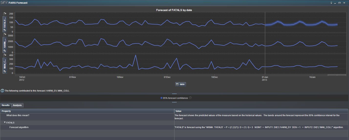
SAS Visual Analytics 7.3 lets you forecast quickly and easily. It is fairly foolproof, and lets you get a quick and dirty forecast with little statistical knowledge.
You can also try to improve your forecast accuracy by adding measures as underlying factors (independent variables/inputs). The forecasting model evaluates these measures to determine whether they are significant underlying factors or not. If the underlying factors do increase the accuracy of the forecast, then the forecast line is adjusted, and the confidence bands are narrowed.
If your forecast includes underlying factors, then you can apply scenario analysis and goal seeking to the forecast. Scenario analysis enables you to forecast hypothetical scenarios by specifying the future values for one or more underlying factors that contribute to the forecast. For example, if you forecast electricity usage for a state, and air temperature is an underlying factor, then you might use scenario analysis to determine how the future electricity usage would change if the temperature increased or decreased by two percent.
In addition to scenario analysis, you can perform goal seeking. Goal seeking enables you to specify a target value for your forecast measure, and then determine the values of your underlying factors that would be required to achieve the target value. For example, if you forecast the profit of a company, and material cost is an underlying factor, then you might use goal seeking to determine what value for material cost would be required to achieve a 10% increase in profit. Visual Analytics 7.3 lets you use scenario analysis and goal seeking together in the same forecast.
A variety of exponential smoothing and Winters methods models are available including:
- Damped-trend exponential smoothing
- Linear exponential smoothing
- Seasonal exponential smoothing
- Winters method (additive)
- Winters method (multiplicative)
With SAS Visual Analytics 7.3, the user has no control over the method chosen. Remember that VA is a tool for exploring your data, and it is designed to be easy to use for business analysts. If you find interesting forecasting results, you will likely want to move to a tool that allows you more control over the forecasting method, such as Forecast Server or ETS. In this respect, VA is a “gateway drug” to more flexible SAS tools that require more training to use. Once you get a taste of how useful forecasting is, you won’t want to stop until you can get the most accurate and most defensible forecasting possible!
Forecast Server Forecast Server provides large-scale automated forecasting. It is an excellent and easy to use tool. It is one of my favorite of the SAS 9 tools, right up there with Enterprise Miner. If you haven’t yet figured out what to buy your Valentine on February 14, I recommend Forecast Server…it is definitely the way to a statistician’s heart. Either that or a trip to a tropical island. You decide.
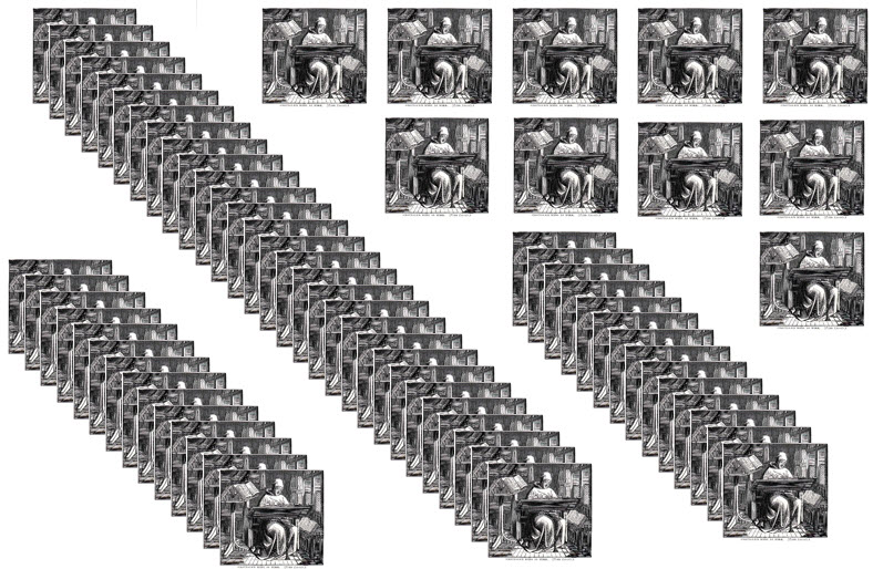
If you are only doing a few forecasts a year, then there is no need for Forecast Server. You can simply use SAS/ETS and programming. I liken this to the monk who has to only copy a few books a year.
However, if you are doing lots of forecasts, for example you are forecasting electricity production for every electric source (petroleum, coal, wind, etc.) and you are forecasting by every state or every country, then you can do one of two things to accomplish your goal: 1. Hire a lot of programmers
OR… 2. Use an automated tool, like Forecast Server
Just a little aside: The first printing was done using ink on carved wooden blocks in China about two thousand years ago. Johannes Gutenberg of Europe invented the Gutenberg printing press around 1440 AD. Automated printing led to mass production of printed materials. This allowed for the broad spread of knowledge and literacy throughout society. The blossoming of the World Wide Web in the 1990s and the invention of iPhones and tablets in the new millennium, have made it easier than ever to spread information. Real-time translation software makes it possible to easily access information written in another language. Indeed, we are living in the Age of Information! Like the printing press allowed for mass production of printed materials, Forecast Server allows for the mass production of forecasting models. Forecast Server uses internal diagnostics to create an endless number of possible models on time-stamped data. It then compares the models to determine which one is the best model, based on the selection criterion that you select. Examples of models are:
- ARIMAs
- Exponential smoothing
- Dampened linear trend
- Croston’s with log transform …and many more…
Forecast Server lets you pick from a whole slew of model selection criteria including mean absolute percent error (MAPE), root mean square error (RMSE), Schwarz Bayesian Criterion (SBC), etc. Holdout samples can be specified so that models are selected not only by how well they fit your training data but also by how well they fit naive data (data not used in building the model).
One drawback is that Forecast Server will not generate multivariate models. Although you can create a bunch of hierarchical models, each with many independent variables, each model has only one dependent variable. Reconciliation of hierarchical models is automatic (and optional) in Forecast Server. HUGE! That means if I am creating a forecast of electricity generation by state and by source, as I move up and down the hierarchy, everything adds up. This is a nice feature that avoids confusion when explaining forecasting results to those managers or accountants who will have your head if numbers don't add up.
But wait...there’s more! Forecast Server generates BASE SAS code! You can easily access this code. And the output for the SAS Forecast Server is generated by ODS (Output Delivery System), which is also part of BASE SAS.
How do I love thee, Forecast Server? Let me count the ways:
- Quick & easy: Forecast Server quickly and automatically creates, fits, and selects forecasting models for you, and new data can be added easily
- Custom models: Your own models can be added to the model repository and compared to Forecast Server’s choices
- Industry knowledge: Explanatory variables, events, etc. based on expert industry knowledge can be used in the model creation
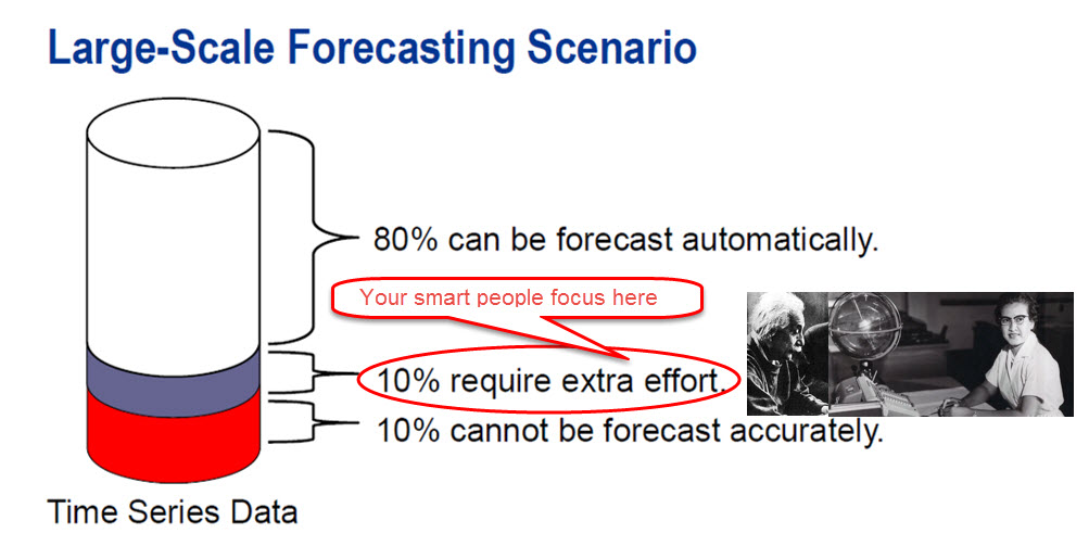
- Focus your resources: 80% of models can be automatically created in Forecast Server, so that your smart statisticians and modelers can focus their time and expertise on tweaking and creating models for high value difficult forecasts
And just in case I haven’t won you over with my raving about Forecast Server, here’s a little summary of features that I developed with help from Terry Woodfield.
Sometimes folks get confused about whether they should use Enterprise Miner or Forecast Server. Forecast Server is strictly for time series data! Meaning you have a historic data set with a time variable.
SAS/STAT and SAS/ETS SAS/ETS software provides SAS procedures that perform econometric and time series analysis and forecasting, as well as financial analysis and reporting. The software also provides an interactive environment for time series forecast and investment analysis. ETS requires significant statistical expertise to use effectively. Only one model is run at a time and automatic batch code was not generated. ETS will let you run multivariate forecasting models! By multivariate, we mean more than one dependent variable.
So there you have it. You CAN predict the future! And speaking of the future, SAS will be releasing new Forecasting software on Viya in 2017. Look for more details on this in the future.
- Mark as Read
- Mark as New
- Bookmark
- Permalink
- Report Inappropriate Content
I have started using SAS University studio lately. Is there any way I can use above syntax related to forecasting in studio?
- Mark as Read
- Mark as New
- Bookmark
- Permalink
- Report Inappropriate Content
SAS AI and Machine Learning Courses
The rapid growth of AI technologies is driving an AI skills gap and demand for AI talent. Ready to grow your AI literacy? SAS offers free ways to get started for beginners, business leaders, and analytics professionals of all skill levels. Your future self will thank you.
- Find more articles tagged with:
- GEL


