- Home
- /
- SAS Communities Library
- /
- An example of Passing-Bablok Regression in SAS
- RSS Feed
- Mark as New
- Mark as Read
- Bookmark
- Subscribe
- Printer Friendly Page
- Report Inappropriate Content
An example of Passing-Bablok Regression in SAS
- Article History
- RSS Feed
- Mark as New
- Mark as Read
- Bookmark
- Subscribe
- Printer Friendly Page
- Report Inappropriate Content
Under the help of @BeverlyBrown , I finally could edit my post . Also thanks the help of @FreelanceReinh
It is SAS code for Passing-Bablok Regression .
P.S. the data I used is stealing from @Rick_SAS blog
https://blogs.sas.com/content/iml/2019/01/07/deming-regression-sas.html
You could find Passing-Bablok Regression is similar with Deming Regression .
data have;
label x="micrograms per deciliter"
      y="kiloOhms";
input x y @@;
datalines;
169.0 45.5 130.8 33.4 109.0 23.8 94.1 19.8 86.3 20.4 78.4 18.7
 76.1 16.1  72.2 16.7  70.0 11.9 69.8 14.6 69.5 10.6 68.7 12.7 67.3 16.9
174.7 57.8 137.9 39.0 114.6 30.4 99.8 21.1 90.1 21.7 85.1 25.2
 80.7 20.6 78.1 19.3  77.8 20.9  76.0 18.2 77.8 18.3 74.2 15.7 73.1 13.9
182.5 55.5 144.0 38.7 123.8 35.1 107.6 30.6 96.9 25.7 92.8 19.2
 87.2 22.4  86.3 18.4  84.4 20.7  83.7 20.6 83.3 20.0 83.9 18.8 82.7 21.8
160.8 49.9 122.7 32.2 102.6 19.2 86.6 14.7 76.1 16.6 69.6 18.8
 66.7  7.4  64.4  8.2  63.0 15.5 61.7 13.7 61.2 9.2 62.4 12.0 58.4 15.2
171.3 48.7 136.3 36.1 111.9 28.6 96.5 21.8 90.3 25.6 82.9 16.8
 78.1 14.1  76.5 14.2  73.5 11.9 74.4 17.7 73.9 17.6 71.9 10.2 72.0 15.6
;


/*创建一个ID变量*/
data temp;
 set have;
 _id+1;
 call symputx('n1',_id); /*样本个数*/
run;

/*计算 Cn^2 组数据的Sij*/
proc sql;
create table temp2 as
select a.x as x1,a.y as y1,b.x as x2,b.y as y2,
case
     when x1 eq x2 and y1 gt y2 then  999999
     when x1 eq x2 and y1 le y2 then -999999
     when x1 ne x2 and y1 eq y2 then 0
	 else (y1-y2)/(x1-x2)
end as Sij
 from temp as a,temp as b
  where a._id<b._id ;
quit;

/*Sij 排除两种情况*/
data temp3;
 set temp2;
 if (x1=x2 and y1=y2) or Sij=-1 then delete;
run;

/*Sij 排序*/
proc sort data=temp3 out=temp4;
by Sij;
run;


proc sql noprint;
/*求有效个数N*/
select count(*) into :n
 from temp4 ;

/*求偏移量K值*/
select count(*) into :k
 from temp4
  where Sij<-1;
quit;
%put &=n &=k ;

/*求斜率的点估计值b  (&slope.) */
data slope;
 set temp4;
 if mod(&n.,2)=1 and _n_ = %eval((&n.+1)/2 + &k.) then output;
 if mod(&n.,2)=0 and _n_ in (%eval(&n./2 + &k.) %eval(&n./2 + 1 + &k.)) then output;
run;
proc sql noprint;
select mean(Sij) into :slope
 from slope;
quit;


/*求斜率的95%置信区间*/
%let alpha=0.05;
data _null_;
 set temp4;
if _n_=1 then do;
 retain Cr M1 M2;
 Cr=quantile('normal',%sysevalf(1-&alpha./2)) * sqrt(&n1.*(&n1.-1)*(2*&n1.+5)/18);
 M1=round((&n.-Cr)/2);
 M2=&n.-M1+1;
 put Cr= M1= M2=;
end;

if _n_=(M1+&k.) then call symputx('slope_lower',Sij);
if _n_=(M2+&k.) then call symputx('slope_upper',Sij);
run;


/*截距估计*/
proc sql noprint;
select median(y-&slope.*x),median(y-&slope_lower.*x),median(y-&slope_upper.*x)
  into :int,:int_lower,:int_upper
 from have;
quit;


/****************打印结果 - print result*********************/
data report;
term='intercept';estimate=&int.;  lower=&int_upper.;  upper=&int_lower.;  output;
term='slope    ';estimate=&slope.;lower=&slope_lower.;upper=&slope_upper.;output;
run;
proc report data=report nowd;
define term/' ';
define estimate/'Estimate';
define lower/"Lower %sysevalf(100*(1-&alpha.))% CI";
define upper/"Upper %sysevalf(100*(1-&alpha.))% CI";
run;


/*  Compare result between Passing-Bablok Regression and Deming regression  */
/*  https://blogs.sas.com/content/iml/2019/01/07/deming-regression-sas.html */
proc sgplot data=have noautolegend;
   scatter x=x y=y;
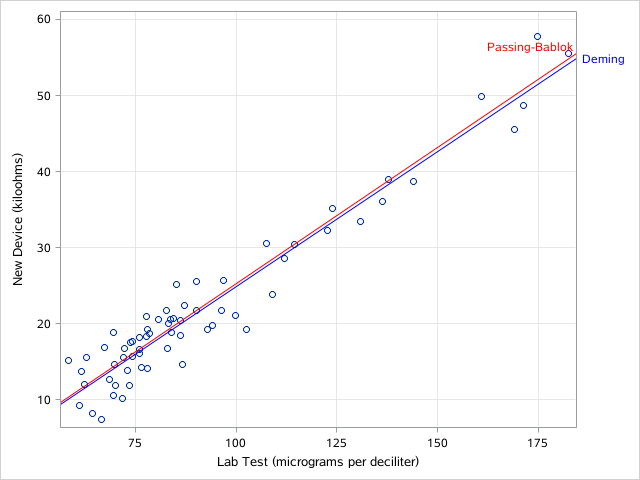
   lineparm x=0 y=-10.56415 slope=0.354463 / clip curvelabel='Deming' curvelabelloc=outside  lineattrs=(color=blue) curvelabelattrs=(color=blue); /* Deming regression estimates */
   lineparm x=0 y=-10.5885  slope=0.358363 / clip curvelabel='Passing-Bablok' lineattrs=(color=red) curvelabelattrs=(color=red); /* Passing-Bablok regression estimates */
   xaxis grid label="Lab Test (micrograms per deciliter)";
   yaxis grid label="New Device (kiloohms)";
run;

- Mark as Read
- Mark as New
- Bookmark
- Permalink
- Report Inappropriate Content
Thanks for posting. I have a half-written article on Passing-Bablock regression that I have been meaning to complete for a long while. As I recall, the issue I struggled with is how to handle repeated measurements. There are subtle issues to think about. Maybe I will be inspired to resume my study.
In addition to the original reference (Passing and Bablok, 1983), the documentation in the NCSS software provides a nice summary:
https://ncss-wpengine.netdna-ssl.com/wp-content/themes/ncss/pdf/Procedures/NCSS/Passing-Bablok_Regre...
- Mark as Read
- Mark as New
- Bookmark
- Permalink
- Report Inappropriate Content
Thank you, @Ksharp, for sharing the code and the interesting original paper. Greatly appreciated. I used Passing-Bablok regression (and also Deming regression) in an earlier job, about 15 years ago, but don't have the SAS code of that time.
As a quick check I've just applied the formulae from the paper to your sample data and obtained slightly different results:
                            Lower      Upper
              Estimate     95% CI     95% CI
  intercept   -10.5777   -13.4906   -7.73623
  slope      0.3582429  0.3254786  0.3905724
Reasons:
- My understanding is that the sign of infinity in the case x1 eq x2 and y1 ne y2 is important (as it affects the ranks of the Sij). There is one pair in the data where minus infinity occurs: x1=x2=76.1, y1=16.1, y2=16.6 (_id=7, 44). Your code sets Sij to 999999 in this case, regardless of the sign. In my code I used the DIVIDE function (which yields .I and .M for +/- infinity, respectively) and then an ORDER BY clause handling the special missing values properly. In your code you could write
case when x1 eq x2 and y1 gt y2 then  999999
     when x1 eq x2 and y1 le y2 then -999999
     ...
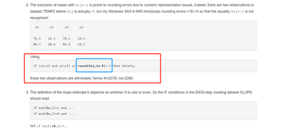
to take the sign into account. - The exclusion of cases with Sij=-1 is prone to rounding errors due to numeric representation issues. Indeed, there are two observations in dataset TEMP2 where Sij is actually -1, but my Windows SAS 9.4M5 introduces rounding errors <1E-14 so that the equality Sij=-1 is not recognized:
 x1      y1      x2      y2

76.1    16.1    78.1    14.1
80.7    20.6    86.6    14.7
Using
if (x1=x2 and y1=y2) or round(Sij,1e-9)=-1 then delete;
those two observations are eliminated, hence N=2078, not 2080. - The definition of the slope estimate b depends on whether N is odd or even. So the IF conditions in the DATA step creating dataset SLOPE should read
if mod(&n,2)=1 and ...
if mod(&n,2)=0 and ...
not if mod(&k,2)=...
- Mark as Read
- Mark as New
- Bookmark
- Permalink
- Report Inappropriate Content
Hi Rick,
My code is very very rough and raw . and I believed there must be many glitch in my code (especially for CI calculating ) .
And I didn't have more example to test my code.
And I am eager to look forwards to your code.
Hope you could post your sas code about Passing-Bablock regression as fast as you could.
I believe many sas users want to have it, include me .
Best !
- Mark as Read
- Mark as New
- Bookmark
- Permalink
- Report Inappropriate Content
Hi FreelanceReinha
Firstly of all ,Thanks for your review. I appreciated . I know there should be some glitch in my code as I said to Rick.
Reasons:
- My understanding is that the sign of infinity in the case x1 eq x2 and y1 ne y2 is important (as it affects the ranks of the Sij). There is one pair in the data where minus infinity occurs: x1=x2=76.1, y1=16.1, y2=16.6 (_id=7, 44). Your code sets Sij to 999999 in this case, regardless of the sign. In my code I used the DIVIDE function (which yields .I and .M for +/- infinity, respectively) and then an ORDER BY clause handling the special missing values properly. In your code you could write
case when x1 eq x2 and y1 gt y2 then  999999
     when x1 eq x2 and y1 le y2 then -999999
     ...
to take the sign into account.
Yes. Yours is better . I took your advice.
Yes. All these three points are really important . Sharp eyes ! Especially the third one , I think I make a big mistake .
The code has been updated .
Hope to see your sas code for Passing-Bablok Regression.
Thank you very much !
Have a nice day !
- Mark as Read
- Mark as New
- Bookmark
- Permalink
- Report Inappropriate Content
I don't know why I would not be able to edit my paper . @BeverlyBrown could help me out ? Replace the first one with this one ?
I would like to thank @FreelanceReinh to find three problems in my code.
So follow @FreelanceReinh 's sharp eyes ,I changed my code and post there .
data have;
label x="micrograms per deciliter"
      y="kiloOhms";
input x y @@;
datalines;
169.0 45.5 130.8 33.4 109.0 23.8 94.1 19.8 86.3 20.4 78.4 18.7
 76.1 16.1  72.2 16.7  70.0 11.9 69.8 14.6 69.5 10.6 68.7 12.7 67.3 16.9
174.7 57.8 137.9 39.0 114.6 30.4 99.8 21.1 90.1 21.7 85.1 25.2
 80.7 20.6 78.1 19.3  77.8 20.9  76.0 18.2 77.8 18.3 74.2 15.7 73.1 13.9
182.5 55.5 144.0 38.7 123.8 35.1 107.6 30.6 96.9 25.7 92.8 19.2
 87.2 22.4  86.3 18.4  84.4 20.7  83.7 20.6 83.3 20.0 83.9 18.8 82.7 21.8
160.8 49.9 122.7 32.2 102.6 19.2 86.6 14.7 76.1 16.6 69.6 18.8
 66.7  7.4  64.4  8.2  63.0 15.5 61.7 13.7 61.2 9.2 62.4 12.0 58.4 15.2
171.3 48.7 136.3 36.1 111.9 28.6 96.5 21.8 90.3 25.6 82.9 16.8
 78.1 14.1  76.5 14.2  73.5 11.9 74.4 17.7 73.9 17.6 71.9 10.2 72.0 15.6
;


/*创建一个ID变量*/
data temp;
 set have;
 _id+1;
 call symputx('n1',_id); /*样本个数*/
run;

/*计算 Cn^2 组数据的Sij*/
proc sql;
create table temp2 as
select a.x as x1,a.y as y1,b.x as x2,b.y as y2,
case
     when x1 eq x2 and y1 gt y2 then  999999
     when x1 eq x2 and y1 le y2 then -999999
     when x1 ne x2 and y1 eq y2 then 0
	 else (y1-y2)/(x1-x2)
end as Sij
 from temp as a,temp as b
  where a._id<b._id ;
quit;

/*Sij 排除两种情况*/
data temp3;
 set temp2;
 if (x1=x2 and y1=y2) or Sij=-1 then delete;
run;

/*Sij 排序*/
proc sort data=temp3 out=temp4;
by Sij;
run;


proc sql noprint;
/*求有效个数N*/
select count(*) into :n
 from temp4 ;

/*求偏移量K值*/
select count(*) into :k
 from temp4
  where Sij<-1;
quit;
%put &=n &=k ;

/*求斜率的点估计值b  (&slope.) */
data slope;
 set temp4;
 if mod(&n.,2)=1 and _n_ = %eval((&n.+1)/2 + &k.) then output;
 if mod(&n.,2)=0 and _n_ in (%eval(&n./2 + &k.) %eval(&n./2 + 1 + &k.)) then output;
run;
proc sql noprint;
select mean(Sij) into :slope
 from slope;
quit;


/*求斜率的95%置信区间*/
%let alpha=0.05;
data _null_;
 set temp4;
if _n_=1 then do;
 retain Cr M1 M2;
 Cr=quantile('normal',%sysevalf(1-&alpha./2)) * sqrt(&n1.*(&n1.-1)*(2*&n1.+5)/18);
 M1=round((&n.-Cr)/2);
 M2=&n.-M1+1;
 put Cr= M1= M2=;
end;

if _n_=(M1+&k.) then call symputx('slope_lower',Sij);
if _n_=(M2+&k.) then call symputx('slope_upper',Sij);
run;


/*截距估计*/
proc sql noprint;
select median(y-&slope.*x),median(y-&slope_lower.*x),median(y-&slope_upper.*x)
  into :int,:int_lower,:int_upper
 from have;
quit;


/****************打印结果 - print result*********************/
data report;
term='intercept';estimate=&int.;  lower=&int_upper.;  upper=&int_lower.;  output;
term='slope    ';estimate=&slope.;lower=&slope_lower.;upper=&slope_upper.;output;
run;
proc report data=report nowd;
define term/' ';
define estimate/'Estimate';
define lower/"Lower %sysevalf(100*(1-&alpha.))% CI";
define upper/"Upper %sysevalf(100*(1-&alpha.))% CI";
run;


/*  Compare result between Passing-Bablok Regression and Deming regression  */
/*  https://blogs.sas.com/content/iml/2019/01/07/deming-regression-sas.html */
proc sgplot data=have noautolegend;
   scatter x=x y=y;
   lineparm x=0 y=-10.56415 slope=0.354463 / clip curvelabel='Deming' curvelabelloc=outside  lineattrs=(color=blue) curvelabelattrs=(color=blue); /* Deming regression estimates */
   lineparm x=0 y=-10.5885  slope=0.358363 / clip curvelabel='Passing-Bablok' lineattrs=(color=red) curvelabelattrs=(color=red); /* Passing-Bablok regression estimates */
   xaxis grid label="Lab Test (micrograms per deciliter)";
   yaxis grid label="New Device (kiloohms)";
run;
- Mark as Read
- Mark as New
- Bookmark
- Permalink
- Report Inappropriate Content
Hello,
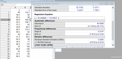
I read your code and found it enlightening. And verified it on Medcalc with your data, but found that the results were slightly different.
But in my ability, I can't tell why the difference is happening, so here's a tip for you to continue your research and look forward to some more research on the code.
- Mark as Read
- Mark as New
- Bookmark
- Permalink
- Report Inappropriate Content
Hello @soulmate and welcome to the SAS Support Communities!
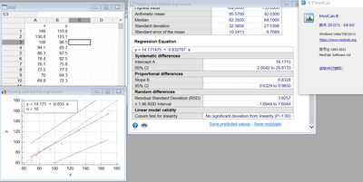
Thanks for bringing MedCalc into play, great idea. My old MedCalc version 9.6.2.0 from 2008 confirms your regression coefficients, but yields different confidence intervals:
Interestingly, these confidence limits are closer to those obtained with SAS.
So we see an example of the well-known fact that even different versions of the same software may produce different results from identical input data.
The current online documentation https://www.medcalc.org/manual/passing-bablok-regression.php mentions a couple of more recent references in addition to the original paper, but doesn't contain any formula for computing the estimates. Further investigation would be needed to find out where the differences come from.
- Mark as Read
- Mark as New
- Bookmark
- Permalink
- Report Inappropriate Content
I found if I used
if (x1=x2 and y1=y2) or Sij=-1 then delete;
would get exactly the result with yours , Surprise ?
So I am thinking whether to use my original code or yours ROUND() function . What your opinion ?
About confident interval , I think it is about the way to calculate , just like @Rick_SAS 's blog mentioned :
https://blogs.sas.com/content/iml/2019/01/07/deming-regression-sas.html
You might wonder how accurate the parameter estimates are. Linnet (1993) recommends using the jackknife method to answer that question. I have previously explained how to jackknife estimates in SAS/IML, and the following program is copied from that article:
And comments from MVT
If CI is calculated by Bootstrap or Jackknife method, and the result might totally different from my code .
- Mark as Read
- Mark as New
- Bookmark
- Permalink
- Report Inappropriate Content
That's interesting, @Ksharp, thank you. So part of the mystery is cleared up: Your result suggests that MedCalc 9.6.2.0 suffers from the same rounding errors (due to numeric representation issues) as any other software does if no countermeasures (such as proper rounding or a fuzzy comparison) are taken. My opinion is that those countermeasures should be taken because this is the only way to obtain results which are consistent
- with results obtained on other hardware/software platforms
- with results from hand calculation
- with results using other measurement units.
The latter point can be demonstrated easily by multiplying all values in your sample data by 10 (i.e., removing the decimal points). The calculation using the resulting integer values is no longer affected by numeric representation errors. Here's the result for the modified data from MedCalc 9.6.2.0:
With the expected factor 10 in the intercept and its CI this result matches that obtained by SAS using the ROUND function appropriately -- as it should, because using a different measurement unit must not affect the method comparison.
- Mark as Read
- Mark as New
- Bookmark
- Permalink
- Report Inappropriate Content
Thanks for your discussion of this issue. @Ksharp,@FreelanceReinhard
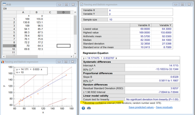
I used MedCalc version 20.026.This is a relatively new software version, and I can understand that @FreelanceReinhard your software version has not yet taken into account the estimation method of the confidence interval.In fact, medcalc already takes into account algorithm updates for confidence intervals.
For confidence interval estimation for PB regression, the Bootstrap or Jackknife method is necessary and scientific.
So, I would like to suggest to you, can you use these two algorithms to optimize your code? @KsharpThis is very important for practitioners in the IVD industry or in the field of medical testing.
As IVD practitioners, and SAS users, it is very desirable to integrate these algorithms on THE SAS without the need to use other statistical software.I wonder what the advice of you two are?
The figure below is medcalc default replocations and random-number seed.
- Mark as Read
- Mark as New
- Bookmark
- Permalink
- Report Inappropriate Content
OK. Here is the code for Bootstrap confident interval . They are very close , but not the same .
Maybe it is due to the algorithm of random sampling ,event the seed is the same. There are a lot of unsure reasons.
Or maybe as @Rick_SAS pointed out :
.As I recall, the issue I struggled with is how to handle repeated measurements.
There are subtle issues to think about.
/*Firstly Make a macro for Passing-Bablok Regression*/
%macro Passing_Bablok_regression(dataset= ,x= ,y= ,SampleID=  );
/*创建一个ID变量*/
data temp(rename=(&x.=x &y.=y));
 set &dataset.;
 _id+1;
 call symputx('n1',_id); /*样本个数*/
run;

/*计算 Cn^2 组数据的Sij*/
proc sql;
create table temp2 as
select a.x as x1,a.y as y1,b.x as x2,b.y as y2,
case when x1 eq x2 and y1 gt y2 then  999999
     when x1 eq x2 and y1 le y2 then -999999
     when x1 ne x2 and y1 eq y2 then 0
	 else (y1-y2)/(x1-x2)
end as Sij
 from temp as a,temp as b
  where a._id<b._id ;
quit;

/*Sij 排除两种情况*/
data temp3;
 set temp2;
 if (x1=x2 and y1=y2) or Sij=-1 then delete;
run;

/*Sij 排序*/
proc sort data=temp3 out=temp4;
by Sij;
run;

proc sql noprint;
/*求有效个数N*/
select count(*) into :n
 from temp4 ;
/*求偏移量K值*/
select count(*) into :k
 from temp4
  where Sij<-1;
quit;
%put &=n &=k ;

/*求斜率的点估计值b  (&slope.) */
data slope;
 set temp4;
 if mod(&n,2)=1 and _n_ = %eval((&n+1)/2 + &k) then output;
 if mod(&n,2)=0 and _n_ in (%eval(&n/2 + &k) %eval(&n/2 + 1 + &k)) then output;
run;
proc sql noprint;
select mean(Sij) into :slope
 from slope;
quit;

/*求斜率的95%置信区间*/
%local alpha;
%let alpha=0.05;
data _null_;
 set temp4;
if _n_=1 then do;
 retain Cr M1 M2;
 Cr=quantile('normal',%sysevalf(1-&alpha./2)) * sqrt(&n1.*(&n1.-1)*(2*&n1.+5)/18);
 M1=round((&n.-Cr)/2);
 M2=&n.-M1+1;
 put Cr= M1= M2=;
end;
if _n_=(M1+&k.) then call symputx('slope_lower',Sij);
if _n_=(M2+&k.) then call symputx('slope_upper',Sij);
run;

/*截距估计*/
proc sql noprint;
select median(y-&slope.*x),median(y-&slope_lower.*x),median(y-&slope_upper.*x)
  into :int,:int_lower,:int_upper
 from temp ;
quit;


/****************Save result*********************/
data report;
SampleID=&SampleID.;
term='intercept';estimate=&int.;  lower=&int_upper.;  upper=&int_lower.;  output;
term='slope    ';estimate=&slope.;lower=&slope_lower.;upper=&slope_upper.;output;
label estimate='Estimate' lower="Lower %sysevalf(100*(1-&alpha.))% CI" upper="Upper %sysevalf(100*(1-&alpha.))% CI";
run;

proc append base=output_pb data=report force;run;
%mend;


data have;
label x="micrograms per deciliter"
      y="kiloOhms";
input x y @@;
datalines;
169.0 45.5 130.8 33.4 109.0 23.8 94.1 19.8 86.3 20.4 78.4 18.7
 76.1 16.1  72.2 16.7  70.0 11.9 69.8 14.6 69.5 10.6 68.7 12.7 67.3 16.9
174.7 57.8 137.9 39.0 114.6 30.4 99.8 21.1 90.1 21.7 85.1 25.2
 80.7 20.6 78.1 19.3  77.8 20.9  76.0 18.2 77.8 18.3 74.2 15.7 73.1 13.9
182.5 55.5 144.0 38.7 123.8 35.1 107.6 30.6 96.9 25.7 92.8 19.2
 87.2 22.4  86.3 18.4  84.4 20.7  83.7 20.6 83.3 20.0 83.9 18.8 82.7 21.8
160.8 49.9 122.7 32.2 102.6 19.2 86.6 14.7 76.1 16.6 69.6 18.8
 66.7  7.4  64.4  8.2  63.0 15.5 61.7 13.7 61.2 9.2 62.4 12.0 58.4 15.2
171.3 48.7 136.3 36.1 111.9 28.6 96.5 21.8 90.3 25.6 82.9 16.8
 78.1 14.1  76.5 14.2  73.5 11.9 74.4 17.7 73.9 17.6 71.9 10.2 72.0 15.6
;


/* 1. Get point estimate of intercept and slope */
proc delete data=Output_pb ;run;
%Passing_Bablok_regression(dataset=have, x=x,y=y ,SampleID=0)
data point_estimate;
 set Output_pb;
 keep term estimate;
run;


/*  The following code for Bootstrap Confidence Interval  is from Rick's blog
https://blogs.sas.com/content/iml/2016/08/10/bootstrap-confidence-interval-sas.html
https://blogs.sas.com/content/iml/2018/06/20/bootstrap-method-example-sas.html      */

%let NumSamples = 1000;       /* number of bootstrap resamples */
/* 2. Generate many bootstrap samples */
proc surveyselect data=have NOPRINT seed=978
     out=BootSSFreq(rename=(Replicate=SampleID))
     method=urs              /* resample with replacement */
     samprate=1              /* each bootstrap sample has N observations */
     OUTHITS                 /* option to suppress the frequency var */
     reps=&NumSamples;       /* generate NumSamples bootstrap resamples */
run;


/* 3. Compute the statistic for each bootstrap sample */
proc freq data=BootSSFreq noprint;
table SampleID/out=SampleID;
run;
proc delete data=Output_pb ;run;
data _null_;
 set SampleID;
 call execute(catt('%nrstr(%Passing_Bablok_regression(dataset=BootSSFreq(where=(SampleID=',SampleID,')) ,x=x ,y=y ,SampleID=',SampleID,'))'));
run;


/* 4. Write stats to BootStats data set */
proc univariate data=Output_pb noprint ; /* use NOPRINT option to suppress output and graphs */
   class  term;
   var estimate ;
   output out=Pctl pctlpre =CI95_
          pctlpts =2.5  97.5       /* compute 95% bootstrap confidence interval */
          pctlname=Lower Upper;
run;


/*Merge the point estimate and Confident Interval together*/
data want;
 merge point_estimate pctl;
 by term;
 label term='09'x estimate='Estimate' CI95_Lower='Lower 95%CI' CI95_Upper='Upper 95%CI';
run;
/*Print resutl*/
proc report data=want nowd; run;
- Mark as Read
- Mark as New
- Bookmark
- Permalink
- Report Inappropriate Content
Thanks for your reply. @Ksharp
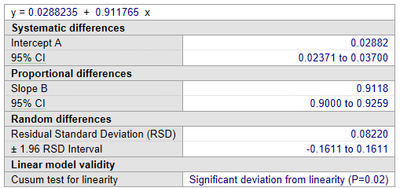
To verify the accuracy of the code more comprehensively, I used a different dataset to verify it.
But different results have been obtained. The point estimates for slope and intercept have been slightly different.
In my opinion, the point estimate does not involve a random sampling algorithm and should be the same, so is there any factor that is not reflected in the code?
SAS result:
MedCalc result:
My data:
data have;
label x="micrograms per deciliter"
y="kiloOhms";
input x y @@;
datalines;
0.07 0.07
0.04 0.10
0.07 0.08
0.05 0.10
0.06 0.08
0.06 0.07
0.03 0.05
0.04 0.05
0.05 0.08
0.05 0.10
0.12 0.21
0.10 0.17
0.03 0.11
0.18 0.24
0.29 0.33
0.05 0.05
0.04 0.05
0.11 0.21
0.38 0.36
0.04 0.05
0.03 0.06
0.06 0.07
0.46 0.27
0.08 0.05
0.02 0.09
0.12 0.23
0.16 0.25
0.07 0.10
0.07 0.07
0.04 0.06
0.11 0.23
0.23 0.21
0.15 0.20
0.05 0.07
0.04 0.14
0.05 0.11
0.17 0.26
8.43 8.12
1.86 1.47
0.17 0.27
8.29 7.71
5.98 5.26
0.57 0.43
0.07 0.10
0.06 0.11
0.21 0.24
8.29 7.84
0.28 0.23
8.25 7.79
0.18 0.25
0.17 0.22
0.15 0.21
8.33 7.67
5.58 5.05
0.09 0.14
1.00 3.72
0.09 0.13
3.88 3.54
0.51 0.42
4.09 3.64
0.89 0.71
5.61 5.18
4.52 4.15
0.09 0.12
0.05 0.05
0.05 0.05
0.04 0.07
0.05 0.07
0.09 0.11
0.03 0.05
2.27 2.08
1.50 1.21
5.05 4.46
0.22 0.25
2.13 1.93
0.05 0.08
4.09 3.61
1.46 1.13
1.20 0.97
0.02 0.05
1.00 1.00
3.39 3.11
1.00 0.05
2.07 1.83
6.68 6.06
3.00 2.97
0.06 0.09
7.17 6.55
1.00 1.00
2.00 0.05
2.91 2.45
3.92 3.36
1.00 1.00
7.20 6.88
6.42 5.83
2.38 2.04
1.97 1.76
4.72 4.37
1.64 1.25
5.48 4.77
5.54 5.16
0.02 0.06
;
run;
- Mark as Read
- Mark as New
- Bookmark
- Permalink
- Report Inappropriate Content
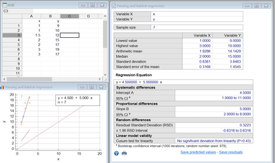
@soulmate I do not have access to MedCalc, but I would be curious to know what answer it gives for each of the following sets of data:
/* only 10 obs */
data Test1;
input x y @@;
datalines;
169.0 155.6 130.8 123.1 109.0  96.5  94.1  85.7 86.3  87.5 78.4 82.5
 76.1  75.6  72.2  77.2  70.0  64.3  69.8  72.3
;

/* repeated data values */
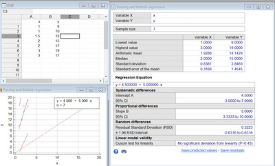
data Test2;
input x y @@;
datalines;
1  9  1 10  1.5 12  2 15  2 17  3 19  3 17
;
- Mark as Read
- Mark as New
- Bookmark
- Permalink
- Report Inappropriate Content
Rick,
I will do it for you .
For the test1 dataset: -- without Bootstrap CI
-- with Bootstrap CI
For the Test2 dataset: -- without Bootstrap CI
-- with Bootstrap CI
- Mark as Read
- Mark as New
- Bookmark
- Permalink
- Report Inappropriate Content
I don't know what to say. I tested another dataset ,and get the exactly the same result.
I guess there are must have some underline adjustment in Medcalc,especially when there are more data ?
data have;
set sashelp.class(keep=weight height rename=(weight=x height=y));
run;
- Mark as Read
- Mark as New
- Bookmark
- Permalink
- Report Inappropriate Content
Thanks for your reply and discussion, after looking at the data today and verifying it with another set of data, I have the following ideas:
1.In method comparison, x and y are usually not much different values and are often used for equivalence analysis.For example, the concentration of glucose in serum is tested with 2 IVD products, so that x and y are very close.
2.The data you used to test your code before, x and y, are very different, which in my opinion is already a significant inconsistency
3.So, this could be the reason why the results are problematic? Maybe MedCalc has its own way of handling similar data?
4.I think (of course, my experience is not enough), the main application area of PB regression is the analysis of laboratory test results,which is regression analysis between two similar data. So this problem is still very important and needs to be solved.
5.Another way of thinking, MedCalc has a built-in way of processing very small data, because many of the previous sets of data are 0.0X, or maybe this causes a slight deviation in the results?
6.I used another set of real data to verify, and the results are as follows(with Bootstrap CI😞
MedCalc:
SAS:
data:
data have;
label x="micrograms per deciliter"
y="kiloOhms";
input x y @@;
datalines;
3.28 3.42
1.91 2.22
15.93 17.45
16.72 17.16
13.83 14.38
1.81 1.94
9.61 8.43
16.06 17.69
16.46 18.10
5.75 7.53
0.053 0.06
17.75 20.28
13.72 15.30
0.857 1.01
14.63 16.08
16.23 15.51
4.42 4.87
2.02 2.33
17.74 19.18
4.12 3.12
15.90 17.16
4.89 5.36
1.65 1.56
21.37 22.71
0.296 0.33
2.66 2.68
11.46 12.07
18.16 16.88
1.85 1.73
11.83 13.61
0.998 1.24
3.80 4.22
6.79 7.85
15.37 18.06
1.37 1.48
8.11 9.88
0.145 0.16
1.63 1.61
6.15 5.88
5.80 5.76
2.41 2.39
17.03 17.32
0.343 0.40
3.75 3.89
8.05 8.95
7.38 6.82
9.76 11.29
3.43 4.24
7.07 8.64
8.46 8.97
6.25 7.24
1.66 1.36
3.98 4.21
9.11 8.08
10.83 11.47
4.66 4.43
8.90 7.89
15.43 15.60
2.87 2.33
0.032 0.03
19.80 21.17
14.92 15.83
6.14 6.68
3.90 4.20
0.132 0.14
0.824 0.92
4.09 4.63
3.22 3.39
7.56 8.13
5.67 6.96
1.53 1.07
5.21 6.58
9.66 8.57
6.48 6.44
1.99 2.29
21.96 22.77
18.08 18.45
11.89 13.24
11.65 11.97
15.02 15.71
0.440 0.42
19.12 20.80
7.13 7.17
16.15 17.54
15.91 17.05
17.76 18.62
11.81 12.12
5.34 5.00
6.19 7.55
5.59 5.66
9.39 9.35
9.45 9.24
6.14 6.67
4.30 4.83
11.46 10.35
3.99 4.34
3.51 3.53
3.33 3.18
9.94 8.58
12.77 14.25
1.56 1.61
11.10 10.56
2.20 2.60
6.12 6.64
8.90 9.79
12.46 14.08
10.05 10.10
0.053 0.05
4.22 3.89
5.76 6.78
1.54 1.06
13.68 14.65
3.42 3.44
2.03 2.46
9.91 12.66
0.832 0.93
2.40 1.88
4.99 6.20
5.90 6.69
0.527 0.59
0.404 0.51
0.450 0.41
0.146 0.15
0.040 0.04
1.23 1.43
5.68 6.31
0.231 0.27
0.254 0.26
0.346 0.38
0.239 0.27
0.311 0.27
3.30 3.22
14.22 13.28
14.18 15.75
0.621 0.53
11.75 12.65
10.32 9.34
15.48 16.43
8.93 7.86
4.05 4.23
11.18 12.65
14.60 15.85
3.76 3.23
9.55 8.99
12.06 11.54
2.00 1.69
11.88 12.07
7.17 7.53
14.54 14.75
5.47 6.34
5.70 5.03
9.69 9.43
0.034 0.03
9.50 9.03
10.35 9.54
0.468 0.44
14.69 15.86
2.57 2.15
1.29 1.22
2.12 1.98
0.061 0.06
12.52 14.54
10.29 12.04
3.42 2.99
1.94 2.04
1.06 0.98
4.61 4.23
3.49 3.22
12.52 14.35
1.29 1.32
6.18 7.12
;
run;
- Mark as Read
- Mark as New
- Bookmark
- Permalink
- Report Inappropriate Content
There is also a small question, why is the same 1000 sampling times, SAS running much slower than MedCalc?
- Mark as Read
- Mark as New
- Bookmark
- Permalink
- Report Inappropriate Content
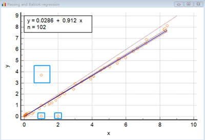
Maybe I found the reason, there are three outliers in data . Medcalc might have skill to handle this situation .
If I delete these outliers .
" if _n_ in (56 83 90) then delete; "
I would get exactly the same result .
@Rick_SAS , Do you know how to handle outliers in this situation as Medcalc?
- Mark as Read
- Mark as New
- Bookmark
- Permalink
- Report Inappropriate Content
"There is also a small question, why is the same 1000 sampling times, SAS running much slower than MedCalc?"
Because I used datastep. If using IML as @Rick_SAS did ,that much be faster .
- Mark as Read
- Mark as New
- Bookmark
- Permalink
- Report Inappropriate Content
Thanks to your reply. I learned a lot from our disscution.
- Mark as Read
- Mark as New
- Bookmark
- Permalink
- Report Inappropriate Content
I have posted a SAS/IML program that performs Passing-Bablok regression and estimates CIs by using the method in the PB paper: Also, an overview and brief discussion of the PB algorithm.
See "Passing-Bablok regression in SAS."
I don't want to hijack this thread, but it is not easy to post code and screenshots in a blog comment, so if you have any comments that involve posting code, feel free to post your feedback here.
- Mark as Read
- Mark as New
- Bookmark
- Permalink
- Report Inappropriate Content
hi Ksharp,long time no see.
I ran the pb regression program again in the past few days and found a problem.
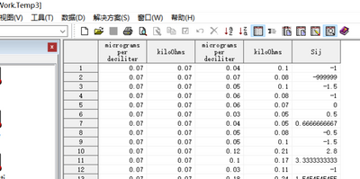
The temp3 dataset needs to delete the sij=-1 observation, but I opened the dataset and still saw the observation with sij=-1.See figure below.
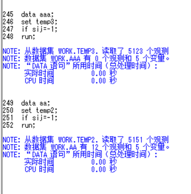
Then I ran the program to see the number of observations sij=-1 in the temp2 and temp3 datasets, and the results were strange.The results show that there is data for sij=-1 in temp2, but no data for sij=-1 in temp3.See figure below.
But this is obviously inconsistent with the dataset results, which should have an impact on the results of the program, right? Why is this happening?
- Mark as Read
- Mark as New
- Bookmark
- Permalink
- Report Inappropriate Content
- Mark as Read
- Mark as New
- Bookmark
- Permalink
- Report Inappropriate Content
soulmate,
Long time no see.
This problem has already mentioned by master @FreelanceReinh . I think it ROUND problem.
I didn't follow @FreelanceReinh 's advice due to comply with software MedCalc . If I used ROUND() ,I would get different result with MedCalc , If I delete ROUND() ,I would get exact result with MedCalc .
- Mark as Read
- Mark as New
- Bookmark
- Permalink
- Report Inappropriate Content
For your second question, &n1. refer to the number of sample, while &n. refer to the VALID number of sample. I think the original paper using the number of sample.
- Mark as Read
- Mark as New
- Bookmark
- Permalink
- Report Inappropriate Content
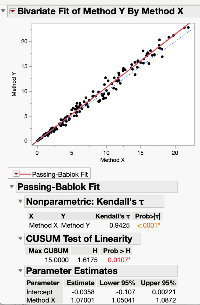
I used your IVD glucose data in your 1/24/22 post with JMP's Passing-Bablok regression tool and it looks like it matches what you're seeing in MedCalc?
Catch up on SAS Innovate 2026
Dive into keynotes, announcements and breakthroughs on demand.
Explore Now →SAS AI and Machine Learning Courses
The rapid growth of AI technologies is driving an AI skills gap and demand for AI talent. Ready to grow your AI literacy? SAS offers free ways to get started for beginners, business leaders, and analytics professionals of all skill levels. Your future self will thank you.


