- RSS Feed
- Mark Topic as New
- Mark Topic as Read
- Float this Topic for Current User
- Bookmark
- Subscribe
- Mute
- Printer Friendly Page
- Mark as New
- Bookmark
- Subscribe
- Mute
- RSS Feed
- Permalink
- Report Inappropriate Content
Hi for all!
I'm seeing powerful of proc optmodel and i would like to resolve svm problem with it. is it possible to resolve support vector machine with it? Like this problem
Suppose we have two vars linearly separable, I know proc svm can do it.
Accepted Solutions
- Mark as New
- Bookmark
- Subscribe
- Mute
- RSS Feed
- Permalink
- Report Inappropriate Content
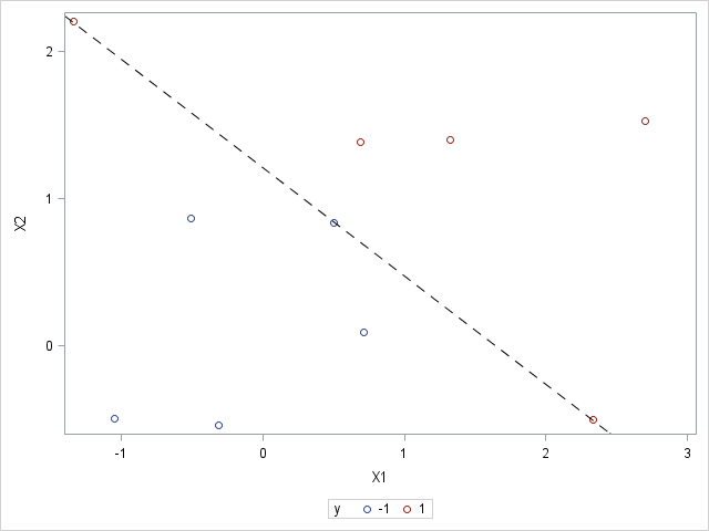
Here's a simple way to do it. I included plots because you have two-dimensional data.
%let n = 2;
data indata;
   input X1 X2 y;
   datalines;
0.49922066	0.834590569	-1
-0.509598752	0.865356638	-1
-0.313012311	-0.54000741	-1
0.713675823	0.094540165	-1
-1.05062909	-0.493905705	-1
1.326427551	1.400617167	1
0.688668461	1.385509561	1
2.705730511	1.526311825	1
2.335457445	-0.497797479	1
-1.340637901	2.205443013	1
;

proc sgplot data=indata;
   scatter x=x1 y=x2 / group=y;
run;

proc optmodel;
   /* read input */
   set OBS;
   num n = &n;
   num x {OBS, 1..n}, y {OBS};
   read data indata into OBS=[_N_] {j in 1..n} <x[_N_,j]=col('x'||j)> y;

   /* declare optimization model */
   var W {1..n};
   var B;
   min Z = 0.5 * sum {j in 1..n} W[j]^2;
   con Separate {i in OBS}:
      y[i] * (sum {j in 1..n} x[i,j]*W[j] - B) >= 1;

   /* call QP solver */
   solve;

   /* plot output */
   num slope = -W[1].sol/W[2].sol;
   num intercept = B.sol/W[2].sol;
   submit slope intercept;
      proc sgplot data=indata;
         scatter x=x1 y=x2 / group=y;
         lineparm x=0 y=&intercept slope=&slope / lineattrs=(pattern=dash color=black);
      run;
   endsubmit;
quit;

- Mark as New
- Bookmark
- Subscribe
- Mute
- RSS Feed
- Permalink
- Report Inappropriate Content
PROC OPTMODEL doesn't has a SVM algorithm. It has transitive closure, shortest path, minimum cost network flow, minimum spanning tree, minimum cut, TSP, among others, but not SVM. For SVM you need to use Enterprise Miner or Viya VDMML.
- Mark as New
- Bookmark
- Subscribe
- Mute
- RSS Feed
- Permalink
- Report Inappropriate Content
Although PROC OPTMODEL does not have anything built-in for SVM, you can formulate the quadratic programming (QP) problem and call the QP solver.
- Mark as New
- Bookmark
- Subscribe
- Mute
- RSS Feed
- Permalink
- Report Inappropriate Content
Suposse we have this data:
 X1	          X2            y
0.49922066	0.834590569	-1
-0.509598752	0.865356638	-1
-0.313012311	-0.54000741	-1
0.713675823	0.094540165	-1
-1.05062909	-0.493905705	-1
1.326427551	1.400617167	1
0.688668461	1.385509561	1
2.705730511	1.526311825	1
2.335457445	-0.497797479	1
-1.340637901	2.205443013	1
how can we apply proc optmodel?
- Mark as New
- Bookmark
- Subscribe
- Mute
- RSS Feed
- Permalink
- Report Inappropriate Content
It seems this data is not related to optimization problem, such as minimize or maximize y. It seems to be a very traditional classification problem, and then you should use the traditional SVM algorithm.
- Mark as New
- Bookmark
- Subscribe
- Mute
- RSS Feed
- Permalink
- Report Inappropriate Content
You right Rob. I was thinking about OPTNET.
- Mark as New
- Bookmark
- Subscribe
- Mute
- RSS Feed
- Permalink
- Report Inappropriate Content
but i dont know how can i do it with my data
- Mark as New
- Bookmark
- Subscribe
- Mute
- RSS Feed
- Permalink
- Report Inappropriate Content
Here's a simple way to do it. I included plots because you have two-dimensional data.
%let n = 2;
data indata;
   input X1 X2 y;
   datalines;
0.49922066	0.834590569	-1
-0.509598752	0.865356638	-1
-0.313012311	-0.54000741	-1
0.713675823	0.094540165	-1
-1.05062909	-0.493905705	-1
1.326427551	1.400617167	1
0.688668461	1.385509561	1
2.705730511	1.526311825	1
2.335457445	-0.497797479	1
-1.340637901	2.205443013	1
;

proc sgplot data=indata;
   scatter x=x1 y=x2 / group=y;
run;

proc optmodel;
   /* read input */
   set OBS;
   num n = &n;
   num x {OBS, 1..n}, y {OBS};
   read data indata into OBS=[_N_] {j in 1..n} <x[_N_,j]=col('x'||j)> y;

   /* declare optimization model */
   var W {1..n};
   var B;
   min Z = 0.5 * sum {j in 1..n} W[j]^2;
   con Separate {i in OBS}:
      y[i] * (sum {j in 1..n} x[i,j]*W[j] - B) >= 1;

   /* call QP solver */
   solve;

   /* plot output */
   num slope = -W[1].sol/W[2].sol;
   num intercept = B.sol/W[2].sol;
   submit slope intercept;
      proc sgplot data=indata;
         scatter x=x1 y=x2 / group=y;
         lineparm x=0 y=&intercept slope=&slope / lineattrs=(pattern=dash color=black);
      run;
   endsubmit;
quit;

- Mark as New
- Bookmark
- Subscribe
- Mute
- RSS Feed
- Permalink
- Report Inappropriate Content
if we have non-separable data, how can we modify our problem?
- Mark as New
- Bookmark
- Subscribe
- Mute
- RSS Feed
- Permalink
- Report Inappropriate Content
   num c = 1e4;
   var W {1..n};
   var B;
   var E {OBS} >= 0;
   min Z = 0.5 * sum {j in 1..n} W[j]^2 + c * sum {i in OBS} E[i];
   con Separate {i in OBS}:
      y[i] * (sum {j in 1..n} x[i,j]*W[j] - B) >= 1 - E[i];
The choice of c is up to you.
- Mark as New
- Bookmark
- Subscribe
- Mute
- RSS Feed
- Permalink
- Report Inappropriate Content
One more question!
Its easy to see how we can classify obs in 2d graph, but if we have five variables (5d), we cant paint it.
Then how can i see how classify my model? for future obs? I know qe can solve this problem with this code but i dont know how translate it.
%let n = 5;
data indata;
input x1 x2 x3 x4 x5 y @@;
datalines;
3.435937542	1.910389226	0.276850846	0.364419827	0.140722091	1
1.752885649	1.190057355	0.599295002	0.227447953	0.815532861	1
1.621776734	1.179003553	0.760496315	0.624320514	0.230451018	1
2.575575289	2.999259474	0.620989763	0.828880959	0.034141306	1
1.568690442	1.864722267	0.410446021	0.977573713	0.837272457	1
2.008282532	2.035882912	0.967093924	0.725730786	0.528795923	1
3.150476337	-0.211155573 0.633565936	0.767706516	0.274370632	1
2.412125188	2.459121555	0.40247943	0.205630191	0.303806821	1
2.886648426	1.458100781	0.661861202	0.822914202	0.314037231	1
2.832672695	3.166103391	0.635750146	0.415985331	0.518241769	1
5.435937542	3.910389226	0.220233529	0.909811353	0.611028911	-1
3.752885649	3.190057355	0.090459485	0.686435643	0.218221874	-1
3.621776734	3.179003553	0.797479778	0.201698903	0.062966533	-1
4.575575289	4.999259474	0.344128219	0.054420354	0.009042683	-1
3.568690442	3.864722267	0.748489181	0.989565182	0.4580315	-1
4.008282532	4.035882912	0.460437955	0.287010879	0.200715865	-1
5.150476337	1.788844427	0.155870021	0.000179874	0.993454689	-1
4.412125188	4.459121555	0.543481598	0.639162032	0.571248807	-1
4.886648426	3.458100781	0.400991393	0.274163115	0.118862113	-1
4.832672695	5.166103391	0.333071111	0.391013648	0.446375253	-1

;
run;

proc optmodel;
 /* read input */
 set OBS;
 num n = &n;
 num x {OBS, 1..n}, y {OBS};
 read data indata into OBS=[_N_] {j in 1..n} <x[_N_,j]=col('x'||j)> y;

 /* declare optimization model */
 var W {1..n};
 var B;
 min Z = 0.5 * sum {j in 1..n} W[j]^2;
 con Separate {i in OBS}:
 y[i] * (sum {j in 1..n} x[i,j]*W[j] - B) >= 1;

 /* call QP solver */
 solve;
 quit;
- Mark as New
- Bookmark
- Subscribe
- Mute
- RSS Feed
- Permalink
- Report Inappropriate Content
You can use the SIGN function to compute on which side of the hyperplane the point lies:
   /* create output */
   create data outdata(drop=i) from [i] {j in 1..n} <col('x'||j)=x[i,j]> y
      yhat=(sign(sum {j in 1..n} x[i,j]*W[j] - B));
- Mark as New
- Bookmark
- Subscribe
- Mute
- RSS Feed
- Permalink
- Report Inappropriate Content
I think you showed all details about solving svm as quadratic programing.
My last question is if we have non-linear case, how we should transform the problem?
thank you very much about your help!
- Mark as New
- Bookmark
- Subscribe
- Mute
- RSS Feed
- Permalink
- Report Inappropriate Content
I just saw Rob has replied the code for proc optmodel.
Here is the code for proc svm.
data x1x2y;
input x1 x2 y;
datalines;
0.49922066 0.834590569 -1
-0.509598752 0.865356638 -1
-0.313012311 -0.54000741 -1
0.713675823 0.094540165 -1
-1.05062909 -0.493905705 -1
1.326427551 1.400617167 1
0.688668461 1.385509561 1
2.705730511 1.526311825 1
2.335457445 -0.497797479 1
-1.340637901 2.205443013 1
run;
proc dmdb batch
data=x1x2y
dmdbcat=_cat
out=_x1x2y;
var x1 x2;
class y;
run;
proc svm
data=_x1x2y
dmdbcat=_cat
kernel=polynom
c=1
k_par=2;
var x1 x2;
target y;
run;
and the results:
| The SAS System |
| ---Start Training: Technique= FQP--- |
| Bias -0.163379279 Applied on Predicted Values |
| The SAS System |
| Classification Table (Training Data) | |||
|---|---|---|---|
| Misclassification=0 Accuracy= 100.00 | |||
| Observed | Predicted | ||
| -1 | 1 | Missing | |
| -1 | 5.0000 | 0 | 0 |
| 1 | 0 | 5.0000 | 0 |
| Missing | 0 | 0 | 0 |
| The SAS System |
| Support Vector Classification | C_CLAS |
|---|---|
| Kernel Function | Polynomial |
| Kernel Function Parameter 1 | 2.000000 |
| Estimation Method | FQP |
| Number of Observations (Train) | 10 |
| Number of Effects | 2 |
| Regularization Parameter C | 1.000000 |
| Classification Error (Training) | 0 |
| Objective Function | -2.925242 |
| Inf. Norm of Gradient | 9.436896E-16 |
| Squared Euclidean Norm of w | 2.983253 |
| Geometric Margin | 1.157937 |
| Number of Support Vectors | 6 |
| Number of S.Vector on Margin | 3 |
| Bias | -0.163379 |
| Norm of Longest Vector | 3.000000 |
| Radius of Sphere Around SV | 2.407486 |
| Estimated VC Dim of Classifier | 18.290903 |
| KT Threshold | . |
| Number of Kernel Calls | 189 |
- Mark as New
- Bookmark
- Subscribe
- Mute
- RSS Feed
- Permalink
- Report Inappropriate Content
dont we use linear kernel?
- Ask the Expert: How to Supercharge Enterprise Agentic Workflows With SAS Retrieval Agent Manager | 05-Feb-2026
- Ask the Expert - Génération de données synthétiques : innovation et confidentialité | 10-Feb-2026
- Ask the Expert: Implementing a Digital Twin for the Monopoly Board Game Using SAS® Viya® | 12-Feb-2026
- SAS CI360 Tips and Tricks: Quick Wins, Shortcuts and Hidden Features Every Marketer Should Know | 17-Feb-2026
- SAS Bowl LIX, Integrating SAS and Git | 18-Feb-2026
- Ask the Expert: Welcome to SAS® Viya® | 19-Feb-2026
- Ask the Expert: How Can SAS Viya Copilot Help Me Build Better Models? | 24-Feb-2026


