- Home
- /
- Programming
- /
- Graphics
- /
- proc gchart, vbar, fill/3d options + line chart
- RSS Feed
- Mark Topic as New
- Mark Topic as Read
- Float this Topic for Current User
- Bookmark
- Subscribe
- Mute
- Printer Friendly Page

- Mark as New
- Bookmark
- Subscribe
- Mute
- RSS Feed
- Permalink
- Report Inappropriate Content
OK Sanjay
I am back with a new twist on the proc template.
So now I have grouped variables-Yet I am having some difficulty dictating the colors-
I have defined the template as:
proc template;
define style Styles.Mydefault;
parent=Styles.Default;
style Graphdata1 /Color=green;
style Graphdata2 /Color=red;
end;
Yet I when add the next part and define the FILLATTRS aspect, it askes for a dynamic or constant value. How do I substitute the Graphdatan components?
into the statement
barchart x=role2 y=comply / skin=modern /*FILLATTRS =(color=Mydefault)*/ discreteoffset=-0.3 barwidth=.8 GROUP=COLOR_SCHEME
name='COMPLIANCE';
One more question BTW-
DO you know where there is a list of all the "skins"? I cannot find one anywwhere.
Thanks again.
Lawrence

- Mark as New
- Bookmark
- Subscribe
- Mute
- RSS Feed
- Permalink
- Report Inappropriate Content
All you need to do is use this new style with the ODS destination you are writing to as follows:
ods listing style=Styles.Mydefault;
proc sgrender data= template= ;
run;
With SAS 9.2, only two "skins" are available: Modern and Satin. There are more with SAS 9.3.
In general, it may be preferable to derive the style element from existing style element so you will also get the other attributes that you are not changing:
style Graphdata1 from Graphdata1 / Color=green;
- Mark as New
- Bookmark
- Subscribe
- Mute
- RSS Feed
- Permalink
- Report Inappropriate Content
Sanjay-OK that works! Thanks.
However when I attempt to output in a PDF or RTF it does not render the colors correctly.
Lawrence
- Mark as New
- Bookmark
- Subscribe
- Mute
- RSS Feed
- Permalink
- Report Inappropriate Content
Did you use the STYLE= option with the PDF and/or RTF destination?
- Mark as New
- Bookmark
- Subscribe
- Mute
- RSS Feed
- Permalink
- Report Inappropriate Content
That works. Thank you again.
- Mark as New
- Bookmark
- Subscribe
- Mute
- RSS Feed
- Permalink
- Report Inappropriate Content
Sanjay,
Because I like to push the limit I am back again w/ more questions on the GTL.
This time I am using the secondary x axis.
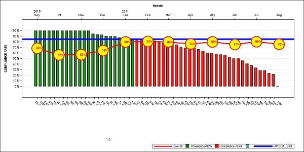
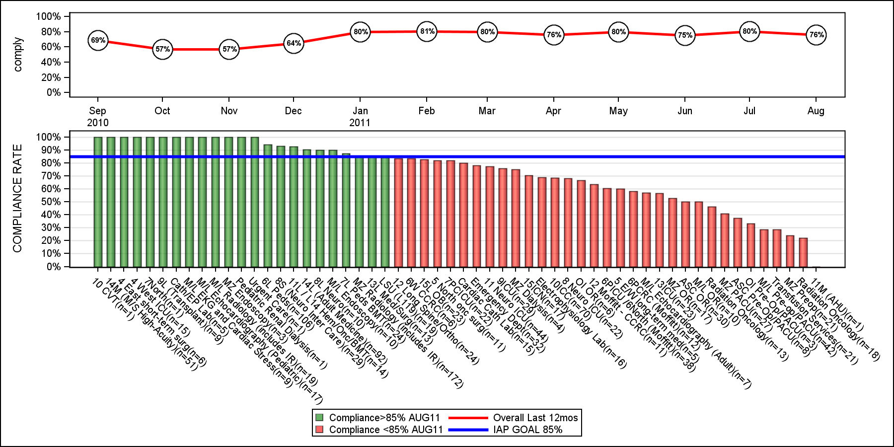
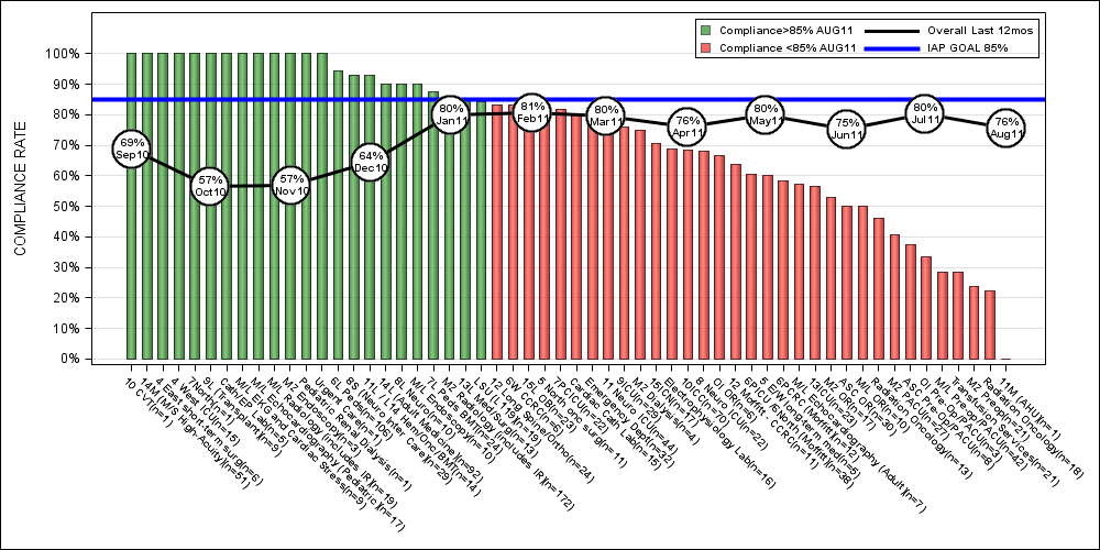
What I am attempting to do is shift the secondary x axis to the bottom but above the units (I have hacked the unit names for security purposes), change the format to a monyy5. format. I have been attempting to use the DISPLAYSECONDARY function without much success. The other option is to place the months in the yellow circle w/ the rate if there is someway to split the text into two lines. I attempted this as well without much success.
The other glitch I have is that it produces a thrid unwanted key in the legend due to the data set structure of the overlay of the datasets so that the units essentially get a blank value for group value. I am not sure how to clear this out.
Both the template code and the image is included that hopefully can help you help me.
Thanks again for your assistance.
Lawrence
define statgraph BarLineMultCo;
begingraph;
;
layout overlay / xaxisopts=(display=(line ticks tickvalues)) cycleattrs=true yaxisopts=(LABEL=('COMPLIANCE RATE') griddisplay=on linearopts=(tickvaluesequence=(start=0 end=1 increment=.1))) ;
barchart x=location y=comply / skin=modern discreteoffset=-0.3 barwidth=.6 /*FILLATTRS =(color=LIPGR)*/GROUP=COLOR_SCHEME
name='COMPLIANCE' legendlabel='COMPLIANCE';
ReferenceLine y=.85 / clip=true Lineattrs=( Pattern=solid thickness=4 color=blue) name="IAP GOAL 85%" legendlabel="IAP GOAL 85%";
seriesplot x=fixdate y=comply / lineattrs=graphdatadefault(thickness=3 color=red) name="Overall" LEGENDLABEL="Overall" xaxis=x2;
scatterplot x=fixdate y=comply / markerattrs=(symbol=circlefilled size=30 color=yellow) xaxis=x2 /*name="Overall" LEGENDLABEL="Overall"*/;
scatterplot x=fixdate y=comply / markerattrs=(symbol=circle size=31 color=red) xaxis=x2 ;
scatterplot x=fixdate y=comply / markercharacter=comply discreteoffset= -0.2 markercharacterattrs=(color=red weight=bold) xaxis=x2;
discretelegend "Overall" "COMPLIANCE" "IAP GOAL 85%" / location=outside halign=right valign=bottom;
endlayout;
endgraph;
end;
run;
- Mark as New
- Bookmark
- Subscribe
- Mute
- RSS Feed
- Permalink
- Report Inappropriate Content
If you can attach the cleaned up data set with code that I can run, it would be a bit easier. The image is very small and a bit fuzzy, so I cannot see the details.
In your code, the bar chart (x=location) is associated with x-axis. The series and scatter (x=fixdate) are associated with x2axis. Since both X & X2 axes are in use, you cannot have secondary axes. Also, this is an interesting combination overlaying two completely different variables.
Bar chart has a group variable with 2 values. So you get the "overall", the 2 values for bar chart and 85% entries in the legend. Which one do you not want?
It is not clear to me exactly what you want to do with the axis or the bubbles.
- Mark as New
- Bookmark
- Subscribe
- Mute
- RSS Feed
- Permalink
- Report Inappropriate Content
Sanjay;
I will upload the code so you can run it in whole and a little further in depth explanation on the issue.
Thanks.
- Mark as New
- Bookmark
- Subscribe
- Mute
- RSS Feed
- Permalink
- Report Inappropriate Content
Sanjay,
Can I send you data set in an excel spreadsheet or csv file?
Just easier than attempting to recreate the entire set to post?
Thanks.
Lawrence.
- Mark as New
- Bookmark
- Subscribe
- Mute
- RSS Feed
- Permalink
- Report Inappropriate Content
Sure.
- Mark as New
- Bookmark
- Subscribe
- Mute
- RSS Feed
- Permalink
- Report Inappropriate Content
Sanjay,
Can you send me an email to Lawrence.Block@ucsfmedctr.org or post your actual email address so I can send you the data.
Thank you.
Lawrence
- Mark as New
- Bookmark
- Subscribe
- Mute
- RSS Feed
- Permalink
- Report Inappropriate Content
Possible solutions:

- Mark as New
- Bookmark
- Subscribe
- Mute
- RSS Feed
- Permalink
- Report Inappropriate Content
Hello Robert,
I would like to make bar chart in SAS for each states for 10-12 different levels. I am trying out this oilbar code for my AmbulatoryClassificationGroupdata to make a bar chart for each state (on x-axis). On y-axis, bar chart for AverageTotalPayments(in dollars) and bars are stacked by each AmbulatoryClasslevels (e.g. 20,73,74,203,209...ans so on). Mt data looks like:
%let name=toplevels;
filename odsout '.';

data my_data;
/**ZCTA5CE10_char=put(ZCTA5CE10, 5.);
	AverageTotalPayments_num=INPUT(AverageTotalPayments, 8.0);
	drop ZCTA5CE10;
	rename ZCTA5CE10_char=ZCTA5CE10;**/
length ProviderState 3.;
input AmbPaymentClassGroup	AverageTotalPayments	ProviderState;
datalines;
209	997.48	AK
209	994.03	AK
209	914.02	AK
209	910.51	AK
209	910.33	AK
377	838.21	AK
377	829.47	AK
377	769.66	AK
377	759.25	AK
207	685.33	AK
270	618.05	AK
207	588.85	AK
269	478.25	AK
269	439.16	AK
269	438.97	AK
269	438.94	AK
336	426.42	AK
269	417.8	AK
336	416.16	AK
336	415.56	AK
336	395.76	AK
336	385.62	AK
73	371.43	AK
336	370.12	AK
74	1158.69	AL
74	1156.78	AL
74	1140.92	AL
74	1089.54	AL
203	780.95	AL
203	761.73	AL
209	753.17	AL
203	753.05	AL
209	751.34	AL
209	730.52	AL
209	724.84	AL
209	723.66	AL
209	723.23	AL
209	722.26	AL
209	717.9	AL
209	715.77	AL
209	715.08	AL
209	714.3	AL
209	712.21	AL
209	710.73	AL
203	709.26	AL
209	708.92	AL
209	708.17	AL
209	706.25	AL
209	705.71	AL
209	705.48	AL
209	705.25	AL
209	701.81	AL
209	701.53	AL
209	699.17	AL
209	699.02	AL
209	698.18	AL
209	697.15	AL
209	696.06	AL
209	690.74	AL
209	679.72	AL
209	679.29	AL
209	678.25	AL
209	677.86	AL
209	675.01	AL
209	673.37	AL
209	669.32	AL
209	667.67	AL
209	666.06	AL
209	665.21	AL
209	664.81	AL
209	664.47	AL
209	661.38	AL
209	661.03	AL
209	660.89	AL
209	660.04	AL
209	657.77	AL
377	655.29	AL
209	651.08	AL
209	649.14	AL
209	648.23	AL
209	647.54	AL
209	644.5	AL
209	643.13	AL
209	641.6	AL
209	640.63	AL
377	638.34	AL
209	631.15	AL
209	628.83	AL
377	621.1	AL
377	613.98	AL
377	609.75	AL
377	608.9	AL
377	608.34	AL
377	608.23	AL
377	605.47	AL
377	605.3	AL
377	603.42	AL
377	602.91	AL
377	602.65	AL
377	601.01	AL
377	597.23	AL
377	593.81	AL
377	592.76	AL
377	592.73	AL
377	591.78	AL
377	591.3	AL
377	590.79	AL
377	588.96	AL
377	587.13	AL
377	587.13	AL
377	585.34	AL
377	580.64	AL
377	580.44	AL
377	578.75	AL
377	578.55	AL
377	576.99	AL
377	573.57	AL
377	573.35	AL
377	572.93	AL
377	570.74	AL
377	570.38	AL
377	568.32	AL
377	563.16	AL
377	562.37	AL
377	561.94	AL
377	561.83	AL
377	559.95	AL
377	559.07	AL
377	557.73	AL
377	556.55	AL
377	556.36	AL
377	556.34	AL
377	556.16	AL
377	556.07	AL
377	553.64	AL
20	553.32	AL
377	553.17	AL
209	552.73	AL
377	551.82	AL
377	549.95	AL
377	548.99	AL
377	548.61	AL
377	547.46	AL
377	546.57	AL
377	545.21	AL
377	541.93	AL
377	536.14	AL
377	533.6	AL
207	531.83	AL
20	530.6	AL
270	530.34	AL
20	525.62	AL
377	525.58	AL
20	524.22	AL
20	523.39	AL
20	523.14	AL
20	522.19	AL
20	521.88	AL
20	520.49	AL
20	517.59	AL
20	517.52	AL
20	516.84	AL
207	513.52	AL
20	512.57	AL
207	508.43	AL
20	507.3	AL
207	506.89	AL
270	503.63	AL
207	502.31	AL
207	502.27	AL
207	501.98	AL
207	501.64	AL
270	501.06	AL
270	501	AL
270	500.52	AL
207	500.18	AL
270	500	AL
20	497.52	AL
270	496.4	AL
270	496.23	AL
207	495.34	AL
20	494.09	AL
20	494.04	AL
20	493.62	AL
20	492.19	AL
207	491.99	AL
207	490.64	AL
207	490.61	AL
207	489.96	AL
270	487.96	AL
270	487.72	AL
20	487.22	AL
207	486.71	AL
270	486.59	AL
207	486.53	AL
207	484.09	AL
207	483.74	AL
270	482.49	AL
270	481.59	AL
20	481.22	AL
207	480.49	AL
270	480.29	AL
207	479.5	AL
20	478.61	AL
207	478.45	AL
20	476.1	AL
207	475.05	AL
20	475	AL
20	474.89	AL
207	474.36	AL
207	474.36	AL
207	473.9	AL
207	473.89	AL
207	473.88	AL
207	473.74	AL
207	473.68	AL
207	472.94	AL
207	472.49	AL
20	472.13	AL
270	471.78	AL
207	470.46	AL
270	470.25	AL
207	469.97	AL
207	469.69	AL
270	469.37	AL
270	469.07	AL
270	467.96	AL
207	467.61	AL
20	467.6	AL
270	466.89	AL
20	466	AL
270	465.6	AL
207	464.11	AL
270	463.32	AL
207	463.13	AL
207	462.79	AL
207	461.08	AL
270	460.8	AL
207	460.55	AL
207	459.72	AL
207	454.7	AL
207	453.84	AL
207	452.93	AL
207	452.68	AL
207	452.61	AL
270	450.65	AL
207	448.06	AL
270	444.55	AL
207	443.65	AL
207	443.26	AL
207	431.88	AL
207	430.28	AL
207	428.82	AL
207	428.4	AL
269	369.88	AL
269	365.94	AL
269	364.61	AL
269	361.55	AL
74	1276.09	AR
74	1221.06	AR
74	1219.07	AR
74	1166.84	AR
203	820.48	AR
209	793.71	AR
209	773.28	AR
209	771.3	AR
203	758.42	AR
209	758.16	AR
209	752.03	AR
209	749.36	AR
209	747.72	AR
209	742.89	AR
209	740.63	AR
209	734.62	AR
209	730.7	AR
209	728.75	AR
And more data I have attached it. I would like to make stacked bar chart for each states by levels. I have tried above code but it creates WORK.my_data but it prints no data and says all of the columns are numeric. I have got this working by using
proc sgplot data=sashelp.prdsale;
  title 'Actual Sales by Product and Quarter';
  vbar product / response=actual group=quarter dataskin=gloss;
  xaxis display=(nolabel);
  yaxis grid;
  run;
But how do I adjust the graph size? I am having difficulty understanding. Thank you.

- Mark as New
- Bookmark
- Subscribe
- Mute
- RSS Feed
- Permalink
- Report Inappropriate Content
Dear Sanjay,
Sorry to open this topic again, but the code you posted on 13-september-2011 17.31 is exactly what I need!
I need a little help to make it fitting perfectly to my needs:
1. I need to put the variabile P in another scale (a secundary axis, e.g. a % value while A-D are in €)
2. I want to put values of variables A-D on the tops of their bars
Could you help me?
Thank you very much
Regards
Paolo
- « Previous
-
- 1
- 2
- Next »
.jpg")
Catch up on SAS Innovate 2026
Nearly 200 sessions are now available on demand in the Innovate Hub.
Watch Now →Learn how use the CAT functions in SAS to join values from multiple variables into a single value.

Find more tutorials on the SAS Users YouTube channel.
SAS Training: Just a Click Away
Ready to level-up your skills? Choose your own adventure.
-
28 replies
-
09-13-2011 03:26 PM
-
13400 views
-
6 likes
-
5 in conversation
-
