Output out options to visualize model results

[Cruise]

Hi folks:

@Rick_SAS @Reeza  @PGStats @ballardw 

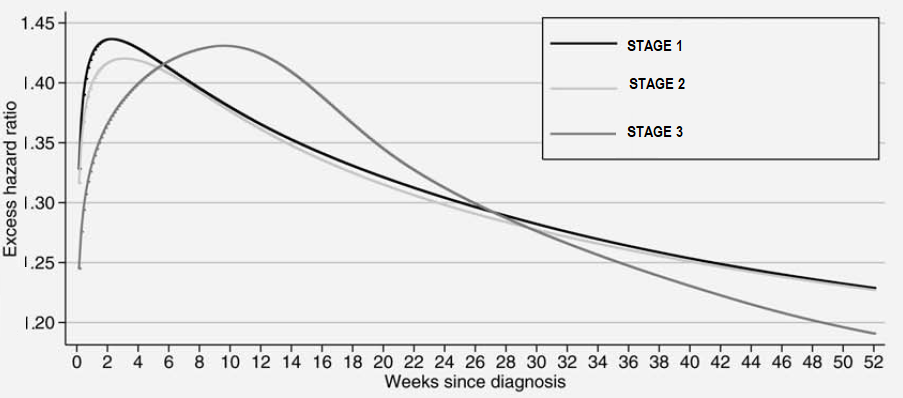
I'm trying to visualize the relationship between follow-up time (fu) on x-axis and excess hazard ratio also known as relative excess risk on y-axis by disease stage.

Desired plot.

The poisson model in the SAS code estimates relative excess risks. I output parameter estimates to a dataset and exponentiated parameter estimates using Dr. Dickman's approach. 

http://www.pauldickman.com/survival/sas/relative_survival_using_sas.pdf

I then plotted exponentiated parameter estimates against the follow-up time grouped by 'stage'. This resulted in the busy plot as shown below. 

ods graphics/width=10in height=3in;
proc sgplot data=parmest;
series x=level1 y=rer /group=stage; 
title 'Excess relative risk by stage, 52 week follow-up';
yaxis label='excess relative risk';
run;

However, the smooth flow line on the plot I want appears to have been produced on the all-record data rather a summary data.

I also, attempted to use effectplot option and got this error from the code below. I'm using SAS 9.4 TS Level 1M5.

NOTE: Algorithm converged.
NOTE: The scale parameter was held fixed.
ERROR: Variable configuration is not currently supported by the EFFECTPLOT statement.
NOTE: The SAS System stopped processing this step because of errors.

ods output parameterestimates=parmest(WHERE=(PARAMETER IN ('fu'))); /* parameter estimates */
proc genmod data=individ order=formatted;
fwdlink link = log(_MEAN_-d_star);
invlink ilink= exp(_XBETA_)+d_star;
class stage;
model d = fu age stage/ error=poisson offset=ln_y type3;
output out=colon.out(keep=xb agegrp fu range stage)  xbeta=xb; 
effectplot /clm moff; 
run;

Variable 'age' is continuous and 'stage' is categorical with 4 levels. 'fu' has 52 levels for 52 weeks of calendar year which is a follow-up interval in this context. 

Below is my full code and mock data attached to the post. 

ods output parameterestimates=parmest;
proc genmod data=have order=formatted;
title3 'Main effects model (first 52 week follow-up, age adjusted, stratified by stage)';
by stage; 
fwdlink link = log(_MEAN_-d_star);
invlink ilink= exp(_XBETA_)+d_star;
class fu;
model d = fu age / error=poisson offset=ln_y type3;
output out=colon.out(keep=xb agegrp fu range stage)  xbeta=xb; 
run;

ods output close;
data parmest; set parmest;
if df gt 0 then do;
rer=exp(estimate);
low_rer=exp(estimate-1.96*stderr);
hi_rer=exp(estimate+1.96*stderr);
end;
run;

proc print data=parmest label noobs;
title4 'Estimates for beta and relative excess risks (RER=exp(beta))';
    id parameter; by parameter notsorted;
    var level1 estimate stderr rer low_rer hi_rer;
    format estimate stderr rer low_rer hi_rer 6.3;
    label
        parameter='Parameter'
        level1='Level'
        estimate='Estimate'
        stderr='Standard Error'
        rer='Estimated RER'
        low_rer='Lower limit 95% CI'
        hi_rer='Upper limit 95% CI';
run;

I'll greatly appreciate your insights on what output methods would help construct the desired plot?

Thanks in advance. Sample data is attached to this post. 

[Cruise]

@Cynthia_sas notification says that you responded to my post. But I couldn't find your comment. I was curious what you would have to say to resolving this problem? I've been reading PROC PHREG output out options. Specifically about outputting martingale residual defining in resmart option. I still am not clear which output dataset contains parameter estimates for all records to be plotted against the follow-up time. 

[Cynthia_sas]

Hi:
I moved the post from where you put it originally into the Graphics forum, since it seemed that most of your questions were graph-related and you'd get more attention in the Graphics Forum.

I am not a stat instructor, my strengths are reporting and ODS.

If you want PDF results, then you need some ODS PDF statements. You seem to have at least one ODS OUTPUT statement for parameter estimates from PROC GENMOD. If you need parameter estimates from PROC PHREG, then you need to look at the PHREG documentation and find out which output object contains parameter estimates. The PHREG doc is here: https://go.documentation.sas.com/?docsetId=statug&docsetTarget=statug_phreg_syntax18.htm&docsetVersi... -- it looks like you're right that RESMART contains the Martingale residual -- if you want those in a separate dataset, then you've got to have an ODS OUTPUT statement for RESMART.

I didn't see PROC PHREG in your posted code.

Cynthia

[Phoenix_LJ]

I am got the same problems , the EFFECTPLOT options only output the pramaters where model's covarance is Discrete variables.However, if there are continuous variables in the model, the parameter estimation cannot be output,

I want to know how to deal this problem!