Graphic help

[samer_badri75]

Greeting All

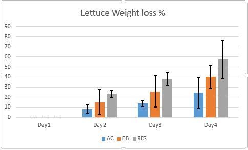
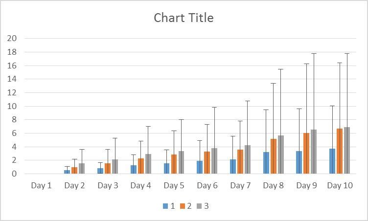
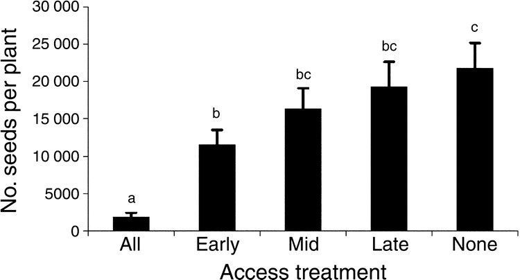
I need hand with SAS 9.4 code, which is related to annotate letters above each midpoint bar of confidence interval .In order to know change in weight loss between the three groups overtime (day).

I used repeated measure SAS.9.4. I attached SAS code, I am  trying  to change the graph to error bars with confidence interval to know  if there is sig different during the day.

Best Regards

Reeza: Note this is related to this other post from earlier today:

https://communities.sas.com/t5/Base-SAS-Programming/SAS-9-4-Code-help/m-p/428633

[ballardw]

Please post code into a code box. Use either the {I} or the "running man" menu icon at the top of the message box.

All you have to do is copy from the editor and paste into the box instead of attaching files.

Did you provide any data in the form of a data step to run or test example code?

[samer_badri75]

* WP;
title2"WP";
data WP;
	input Treatment$ Rep	Day1	Day2	Day3	Day4	Day5	Day6	Day7	Day8	Day9 Day10;
	datalines;
Hybrid	1.00	0.00	0.25	0.52	0.77	0.89	0.89	1.02	1.02	1.02	1.15
Hybrid	2.00	0.00	0.51	0.92	1.13	1.23	1.23	1.43	1.44	1.53	1.53
Hybrid	3.00	0.00	0.33	0.44	0.44	0.66	0.88	0.88	1.32	1.65	2.74
Hybrid	4.00	0.00	0.99	1.58	2.67	3.36	4.73	5.33	9.08	9.27	9.57
Q	    1.00	0.00	0.59	0.69	1.75	1.98	1.98	2.23	2.67	2.78	2.90
Q	    2.00	0.00	0.79	1.24	1.24	1.45	1.80	1.93	2.29	2.73	2.96
Q	    3.00	0.00	0.42	0.72	1.34	1.75	2.26	2.57	2.78	2.88	5.14
Q	    4.00	0.00	2.05	3.49	4.64	6.16	7.04	7.52	12.88	15.68	15.68
Lab	    1.00	0.00	1.34	1.47	1.83	2.07	2.19	2.58	2.95	3.31	3.31
Lab	    2.00	0.00	0.68	0.79	1.24	1.47	1.47	1.57	2.05	2.37	2.60
Lab	    3.00	0.00	0.76	1.31	1.85	2.18	2.18	2.40	2.94	3.48	4.68
Lab	    4.00	0.00	3.42	5.07	6.73	7.71	9.47	10.35	14.85	17.10	17.10

;
run;
* Convert columns of observations to rows - useful for plotting;
data WPplot;
	set WP;
	keep treatment rep Day WP;
	Day=1; WP=Day1; output;
	Day=2; WP=Day2; output;
	Day=3; WP=Day3; output;
	Day=4; WP=Day4; output;
	Day=5; WP=Day5; output;
	Day=6; WP=Day6; output;
	Day=7; WP=Day7; output;
	Day=8; WP=Day8; output;
	Day=9; WP=Day9; output;
	Day=10; WP=Day10; output;
run;
* Print column data set;
proc print data=WPplot;
run;
* Plot observations for each subject through Day;
proc gplot data=WPplot uniform;
	by treatment;
	plot WP*Day=rep;
	symbol1 i=j;
run;
* Plot means for each treatment through Day;
proc gplot data=WPplot;
	plot WP*Day=treatment;
	symbol1 i=std1mjt;
run;
* Profile analysis and repeated measures ANOVA;
proc glm data=WP;
	class treatment;
	model Day1	Day2	Day3	Day4	Day5	Day6	Day7	Day8	Day9 Day10= treatment / nouni;
	repeated Day profile;
run;
* Mixed models analysis;
proc mixed data=WPplot;
	class treatment Day rep;
	model WP = treatment Day treatment*Day / outp=resids;
	* Try type=cs, type=ar(1), or type=un and compare AIC or BIC values.
	  The model with smallest AIC or BIC is the best model;
	repeated / type=cs subject=rep(treatment) rcorr;
run;
quit;

Yes I have data on the example

Many thanks

[Reeza]

If you switch to SGPLOT the TEXT or MARKERCHAR statements are likely what you want. 

SAS/GRAPH quality and capabilities are severely limited in comparison to SGProcedures. There are some things still only possible in SAS/GRAPH but that keeps decreasing.

Also, check the SGPLOT examples, there are few that are probably pretty close to what you want.

[ballardw · Accepted solution]

You don't say which actual variables you want to plot so I guess here:

proc sgplot data=resids;
   scatter x=day  y=pred /group=treatment
      yerrorlower=lower
      yerrorupper=upper
   ;
run;

Which will create errorbars. However the range of your errors in relation to the difference between treatments, if I have the right variables, is such that for this data there might not be enough difference to talk about.

You can place text at the locations of the error bar lines such as:

proc sgplot data=resids;
   scatter x=day  y=pred /group=treatment
      yerrorlower=lower
      yerrorupper=upper
   ;
   text x=day y=upper text=treatment/group=treatment;
run;

Add a separate text variable or one for each of upper and lower if you want different text. the use of group on the TEXT plot is so the color and characteristics make things a bit clearer which text goes with which plot element.

[samer_badri75]

Greeting Sir

Many thanks for your help

I am still looking for the letter on the graph

I attach Doc it have one color graph which is related to my data and the other from a research, I like to add the letter to the error bars of confidence interval to show the differences  in w% during the day. 

Best Regards

Samir

[ballardw]

I don't open DOCX files from unknown sources due to virus and such concerns.

If you have an image, get it as a PNG or GIF or JPEG or similar and then you can insert it into the post with the PHOTOS icon.

The TEXT plot will show any text at given positions. I used the text=treatment as it was in the data set. If you want other text 1) add a variable to your data with the desired location values of an x and y variable.

[samer_badri75]

 many thanks

[Reeza]

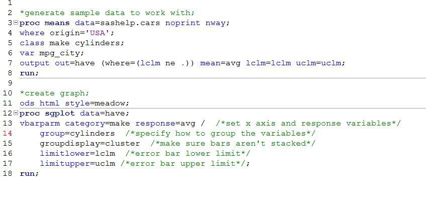
Assuming you have SAS 9.4+ you can use SGPLOT with the VBARPARM and the LIMITLOWER/LIMITUPPER to achieve this relatively painlessly. 

See the image below.

[samer_badri75]

* WP;
title2"WP";
data WP;
	input Treatment$ Rep	Day1	Day2	Day3	Day4	Day5	Day6	Day7	Day8	Day9 Day10;
	datalines;
Ec	1.00	0.00	0.25	0.52	0.77	0.89	0.89	1.02	1.02	1.02	1.15
Ec	2.00	0.00	0.51	0.92	1.13	1.23	1.23	1.43	1.44	1.53	1.53
Ec	3.00	0.00	0.33	0.44	0.44	0.66	0.88	0.88	1.32	1.65	2.74
Ec	4.00	0.00	0.99	1.58	2.67	3.36	4.73	5.33	9.08	9.27	9.57
FB	    1.00	0.00	0.59	0.69	1.75	1.98	1.98	2.23	2.67	2.78	2.90
FB	    2.00	0.00	0.79	1.24	1.24	1.45	1.80	1.93	2.29	2.73	2.96
FB	    3.00	0.00	0.42	0.72	1.34	1.75	2.26	2.57	2.78	2.88	5.14
FB	    4.00	0.00	2.05	3.49	4.64	6.16	7.04	7.52	12.88	15.68	15.68
RES	    1.00	0.00	1.34	1.47	1.83	2.07	2.19	2.58	2.95	3.31	3.31
RES	    2.00	0.00	0.68	0.79	1.24	1.47	1.47	1.57	2.05	2.37	2.60
RES	    3.00	0.00	0.76	1.31	1.85	2.18	2.18	2.40	2.94	3.48	4.68
RES	    4.00	0.00	3.42	5.07	6.73	7.71	9.47	10.35	14.85	17.10	17.10

;
run;
proc means data=sashelp.cars boprint nway;
where origin='USA';
class make cylinders;
var mpg_city;
output out=have (where=lclm ne .)) mean=avg lclm=lclm uclm=uclm;
run;
*create graph;
ods html style=meaow;
proc sgplot data=have;
vbarpam category=make response=avg /   /*set x ais and response variables*/
group=cylinders /*specify how to group the variables*/
groupdisplay=cluster  /*make sure bars aren't stacked*/
limitlower=lclm  /*error bar lower limit*/
limitupper=uclm  /*error nad upper limit*/;
run;

Many thanks for your help

Yes I have SAS 9.4 I print and run it but there is some thing wrong !

[Reeza]

Yes I have SAS 9.4 I print and run it but there is some thing wrong !

It would help a lot if you say what's wrong. 

The code I posted doesn't use your sample data, it's a generic example that uses a SAS data set. Look at the data and the code to determine how it works and change it to match your situation.  

[samer_badri75]

Greeting Sir

I am write the code, but it doesn't work

I m not sure what is the error

Best Regards

Samit

* WP;
title2"WP";
data WP;
	input Treatment$ Rep	Day1	Day2	Day3	Day4	Day5	Day6	Day7	Day8	Day9 Day10;
	datalines;
Ec	1.00	0.00	0.25	0.52	0.77	0.89	0.89	1.02	1.02	1.02	1.15
Ec	2.00	0.00	0.51	0.92	1.13	1.23	1.23	1.43	1.44	1.53	1.53
Ec	3.00	0.00	0.33	0.44	0.44	0.66	0.88	0.88	1.32	1.65	2.74
Ec	4.00	0.00	0.99	1.58	2.67	3.36	4.73	5.33	9.08	9.27	9.57
FB	    1.00	0.00	0.59	0.69	1.75	1.98	1.98	2.23	2.67	2.78	2.90
FB	    2.00	0.00	0.79	1.24	1.24	1.45	1.80	1.93	2.29	2.73	2.96
FB	    3.00	0.00	0.42	0.72	1.34	1.75	2.26	2.57	2.78	2.88	5.14
FB	    4.00	0.00	2.05	3.49	4.64	6.16	7.04	7.52	12.88	15.68	15.68
RES	    1.00	0.00	1.34	1.47	1.83	2.07	2.19	2.58	2.95	3.31	3.31
RES	    2.00	0.00	0.68	0.79	1.24	1.47	1.47	1.57	2.05	2.37	2.60
RES	    3.00	0.00	0.76	1.31	1.85	2.18	2.18	2.40	2.94	3.48	4.68
RES	    4.00	0.00	3.42	5.07	6.73	7.71	9.47	10.35	14.85	17.10	17.10

;
run;
* Convert columns of observations to rows - useful for plotting;
data WPplot;
	set WP;
	keep treatment rep Day WP;
	Day=1; WP=Day1; output;
	Day=2; WP=Day2; output;
	Day=3; WP=Day3; output;
	Day=4; WP=Day4; output;
	Day=5; WP=Day5; output;
	Day=6; WP=Day6; output;
	Day=7; WP=Day7; output;
	Day=8; WP=Day8; output;
	Day=9; WP=Day9; output;
	Day=10; WP=Day10; output;
run;
* Print column data set;
proc print data=WPplot;
run;
* Plot observations for each subject through Day;
proc gplot data=WPplot uniform;
	by treatment;
	plot WP*Day=rep;
	symbol1 i=j;
run;
* Plot means for each treatment through Day;
proc gplot data=WPplot;
	plot WP*Day=treatment;
	symbol1 i=std1mjt;
run;
* Profile analysis and repeated measures ANOVA;
proc glm data=WP;
	class treatment;
	model Day1	Day2	Day3	Day4	Day5	Day6	Day7	Day8	Day9 Day10= treatment / nouni;
	repeated Day profile;
run;
* Mixed models analysis;
proc mixed data=WPplot;
	class treatment Day rep;
	model WP = treatment Day treatment*Day / outp=resids;
	* Try type=cs, type=ar(1), or type=un and compare AIC or BIC values.
	  The model with smallest AIC or BIC is the best model;
	repeated / type=cs subject=rep(treatment) rcorr;
run;
quit;
proc sgplot data=resids;
   vbarparm category=day  response=pred /group=treatment
      groupdisplay=cluster
      limitlower=lower
      limitupper=upper
   ;
run;
proc means data=sashelp.cars noprint nway;
where origin='USA';
class make cylinders;
var mpg_city;
output out=have (where=(lclm ne . )) mean=vag lclm=lclm uclm=uclm;
run;
*creat graph;
ods html style=meadow;
vbarparm category=make response=avg /  /*set x axis and response variables*/
         group=cylinders /*specify how to group the variables*/
		 groupdisplay=cluster  /*make sure bars aren't stacked*/
		 limitlower=lclm /*error bar lower limit*/
		 limitupper=uclm /*error bar upper limit*/;
		 run;

[Reeza]

What does 'doesn't work'?

And I'm not a sir, you really shouldn't assume the gender of people you interact with online. 

[ballardw]

Neither of those graphs point to any variables you referenced in any of your input or output data sets.

I have to assume that you mean to graph from the data set resids created by the procedure output.

However the structure of that data contains a problem for showing a single bar per treatment: The variable REP means that you do not have a single day/predicted value/ upper and lower limit combination to display.

The VBARPARM plot is intended to create bars from summarized data but expects a single record for each combination of category (day), response (predicted value) and group (treatment) variables.

Perhaps you don't actually intend to have REP as a class variable in the Proc code? That creates a separate analysis for each level of REP.

Try rerunning the Proc without rep as a class variable and then look at this:

proc sgplot data=resids;
   vbarparm category=day  response=pred /group=treatment
      groupdisplay=cluster
      limitlower=lower
      limitupper=upper
   ;
run;

You'll likely find that your confidence limits are much narrower as well.

[samer_badri75]

This is related to my data, iput the other one by accident