- Home
- /
- Programming
- /
- Graphics
- /
- Re: Adding a textbox in ODS graphics Designer
- RSS Feed
- Mark Topic as New
- Mark Topic as Read
- Float this Topic for Current User
- Bookmark
- Subscribe
- Mute
- Printer Friendly Page
- Mark as New
- Bookmark
- Subscribe
- Mute
- RSS Feed
- Permalink
- Report Inappropriate Content
Hi everyone,
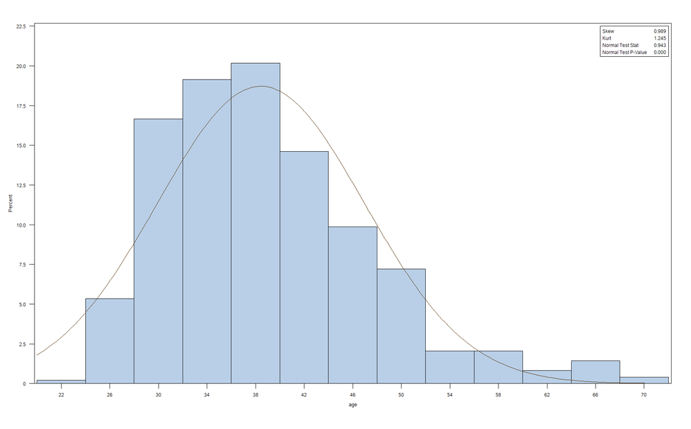
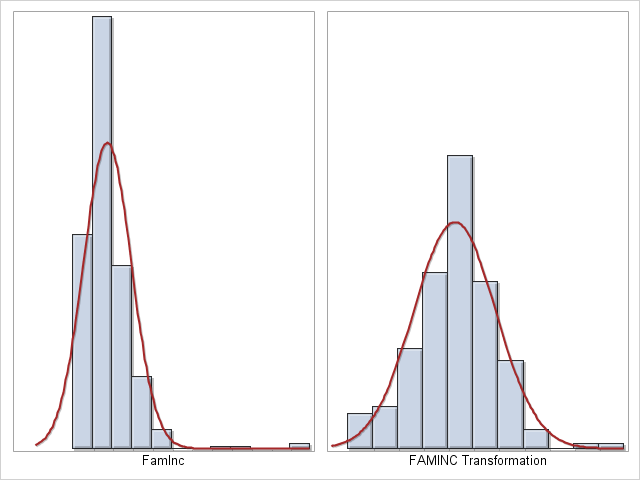
I just discovered ODS Graphics Designer today. It is a really cool tool. I am exploring its capabilities by trying to replicate a histograph I normally generate using Proc Univariate. Using the ODS Graphics Designer, I figured out how to produce two side-by-side histograms with normal overlays. However, I cannot figure out how to add a textbox displaying the skewness, kurtosis, and Shapiro-Wilk values. See attached figures. I am sure this can be accomplished via the ODS Graphics Editor. However, I am looking for a programmatic solution since my ultimate goal is to save the figure as SAS code that can be used as a template. Can someone help or let me know if ODS Graphics Designer does not have the capacity to add textboxes that can be edited similar to the one generated by Proc Univarite.
Thanks,
Cristian
- Mark as New
- Bookmark
- Subscribe
- Mute
- RSS Feed
- Permalink
- Report Inappropriate Content
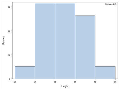
These are called "comparative histograms." You can create them by using PROC UNIVARIATE. Use the CLASS statement and the INSET statement as follows:
proc univariate data=sashelp.class normal;
class sex;
var height;
histogram height;
inset skew kurt normaltest pnormal;
run;
If you decide to use SGPLOT instead, an article that might be helpful is "Comparative histograms: Panel and overlay histograms in SAS"
If you post some sample data, it
- Mark as New
- Bookmark
- Subscribe
- Mute
- RSS Feed
- Permalink
- Report Inappropriate Content
Well, I have reached the conclusion that ODS Graphics Designer cannot add an inset, which is a shame since it produces very nice figures. Hence, I am left to use Proc Univariate.
Rick, I am working on adapting the code you sent but ran into a hickup. Namely, the X axis values are different. Hence, the figures look terrible. I am posting a stacked dataset in case you (or others) have suggestions. Here is what I am trying to achieve. In the left panel I would like to display a histogram of the raw data with a normal overlay while in the right panel I would like to display the BoxCox transformed data. In the stacked dataset source=1 denotes the raw data while source=2 denotes the Box-Cox transformed data. I would also like include insets in both panels reporting the skewness, kurtosis, and Shapiro-Wilk test statistics. It is this last part that I could not get ODS Graphics Designer to do. I can achieve this in individual figures using Proc Univariate but I would like to display them in side-by-side panels. I do not need either the X or Y axis displayed.
thanks,
Cristian
PS, I am posting an Excel file because the discussion board would not let me post a SAS file.
- Mark as New
- Bookmark
- Subscribe
- Mute
- RSS Feed
- Permalink
- Report Inappropriate Content
Then you are NOT doing a comparative histogram. You are just trying to create a panel that contains two histograms.
First, recast the data so that the X and the transformed X data are in different variables (wide form). Then use ODS LAYOUT to specify that you want two graphs side-by-side.
/* gridded layout in HTML, POWERPOINT, and PDF */
ods noproctitle;
ods layout gridded columns=2 advance=table;

ods graphics / height=400px width=400px;
ods select histogram;
proc univariate data=sashelp.class normal;
   histogram height weight;
   inset skew kurt normaltest pnormal;
run;

ods layout end;
For more on the ODS LAYOUT GRIDDED statement, see "Arrange matrices and graphs in a gridded layout"
- Mark as New
- Bookmark
- Subscribe
- Mute
- RSS Feed
- Permalink
- Report Inappropriate Content
Glad to hear you have discovered the ODS Graphics Designer. It is a great tool to create many graphs, and also as a good learning tool for GTL as you can see the generated code under "View->Code". The idea is to get you started, then you can customize by copying the genereated code to the SAS Program Editor code and add the features that are not available in Designer.
You can add a TextBox in Designer to your graph using the "Text Entry" under the "Insets" pane. However, only one text entry is allowed per position as I did below using Designer. I just added some text as an example. To add a block of entries, I suggest you copy the generated GTL code from the View->Code window, and then add a LAYOUT GRIDDED in the upper right corner with 4 rows to display the statistics. Then you can also use macros or dynamics to add the values into the inset.
- Mark as New
- Bookmark
- Subscribe
- Mute
- RSS Feed
- Permalink
- Report Inappropriate Content
Clearly I must not be keeping up with newer developments in SAS as I am unfamiliar with the suggested approaches.
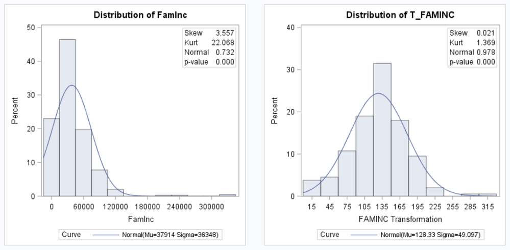
Rick, I adopted your method and it got me nearly all the way there. I am attaching a figure. There are two things that would get me all the way to where I would like to wind up. First, the output was in html. However, I need to be able to save the figure in order to include in a manuscript. I had to crop a screenshot to generate the attached figure. So, is there a way to save a png or emf file? Second, can the legend at the bottom be dropped? I could not locate the option within Proc Univariate.
Sanjay, your approach in intriguing but I need some help to understand how to replicate the inset from Proc Univariate. Below is the code generated by ODS Graphics Designer. How can I use the LAYOUT GRIDDED to add two insets, one to each panel. I attached the dataset to a previous reply.
Much thanks to all,
Cristian
proc template;
define statgraph Graph;
dynamic _FAMINC _T_FAMINC;
begingraph / dataskin=crisp attrpriority=Color;
layout lattice / rowdatarange=union columndatarange=data columns=2 rowgutter=10 columngutter=10 columnweights=(1.0 1.0);
layout overlay / xaxisopts=( display=(LINE LABEL ));
histogram _FAMINC / name='histogram' binaxis=false scale=Percent includemissinggroup=true;
densityplot _FAMINC / name='normal' includemissinggroup=true normal() lineattrs=(color=CXA52829 );
endlayout;
layout overlay / xaxisopts=( display=(LINE LABEL ));
histogram _T_FAMINC / name='histogram2' binaxis=false;
densityplot _T_FAMINC / name='normal2' includemissinggroup=true normal() lineattrs=(color=CXA52829 );
endlayout;
rowaxes;
rowaxis / display=none;
endrowaxes;
endlayout;
endgraph;
end;
run;
proc sgrender data=WORK._TRANSFORMED_ template=Graph;
dynamic _FAMINC="FAMINC" _T_FAMINC="'T_FAMINC'n";
run;
- Mark as New
- Bookmark
- Subscribe
- Mute
- RSS Feed
- Permalink
- Report Inappropriate Content
You will need some knowledge of GTL to add the insets in each cell. I can't see what you want to add, but here is the general process. I think this will work, but you may need to fix any syntax typos. You can use HALIGN= on the entries. See code in bold.
proc template;
define statgraph Graph;
dynamic _FAMINC _T_FAMINC;
dynamic _skew1 _kurt1 _norm1 _p1 _skew2 _kurt2 _norm2 _p2;
begingraph / dataskin=crisp attrpriority=Color;
layout lattice / rowdatarange=union columndatarange=data columns=2 rowgutter=10 columngutter=10 columnweights=(1.0 1.0);
layout overlay / xaxisopts=( display=(LINE LABEL ));
layout gridded / rows=2 columns=2 halign=right valign=top border=true;
entry "Skew"; entry _skew1;
entry "Kurt"; entry _kurt1;
entry "Normal"; entry _norm1;
entry "p-value"; entry _p1;
endlayout;
histogram _FAMINC / name='histogram' binaxis=false scale=Percent includemissinggroup=true;
densityplot _FAMINC / name='normal' includemissinggroup=true normal() lineattrs=(color=CXA52829 );
endlayout;
layout overlay / xaxisopts=( display=(LINE LABEL ));
layout gridded / rows=2 columns=2 halign=right valign=top;
entry "Skew"; entry _skew2;
entry "Kurt"; entry _kurt2;
entry "Normal"; entry _norm2;
entry "p-value"; entry _p2;
endlayout;
histogram _T_FAMINC / name='histogram2' binaxis=false;
densityplot _T_FAMINC / name='normal2' includemissinggroup=true normal() lineattrs=(color=CXA52829 );
endlayout;
rowaxes;
rowaxis / display=none;
endrowaxes;
endlayout;
endgraph;
end;
run;
proc sgrender data=WORK._TRANSFORMED_ template=Graph;
dynamic _FAMINC="FAMINC" _T_FAMINC="'T_FAMINC'n";
/*define dyamics for the stat values*/
run;
- Mark as New
- Bookmark
- Subscribe
- Mute
- RSS Feed
- Permalink
- Report Inappropriate Content
To save the graph as a PNG, you can just right-click in the HTML browser and use "Save picture as..." from the drop-down menu. Or you can Google "sas save ODS graph as PNG".
To suppress the legend from PROC UNIVARIATE, edit the Base.Univariate.Graphics.Histogram template as explained in this thread:
- Mark as New
- Bookmark
- Subscribe
- Mute
- RSS Feed
- Permalink
- Report Inappropriate Content
Sanjay,
I am intrigued to learn more about GTL. Are there some basic resources you can direct me to. I tried your syntax but got an error. Without knowing more about GTL I am not sure how to proceed. Is there a way to see the syntax of existing templates? Perhaps if I saw the syntax for the Univariate histogram with the inset I could figure out how to revise the code. Here is the error that SAS gave me.
Cristian
1058 proc template;
1059 define statgraph ComparativeHistograms;
1060 dynamic _FAMINC _T_FAMINC _FAMINC2 _T_FAMINC2;
1061 dynamic _skew1 _kurt1 _norm1 _p1 _skew2 _kurt2 _norm2 _p2;
1062 begingraph / designwidth=640 designheight=400 backgroundcolor=CXE8E6E8 dataskin=crisp attrpriority=Color;
1063 entrytitle halign=center 'Family Income' / textattrs=(family='Georgia' size=12 style=normal weight=bold );
1064 layout lattice
1065 / rowdatarange=union columndatarange=union rows=2 columns=2 rowgutter=10 columngutter=10 rowweights=(1.0
1065! preferred) columnweights=(1.0 1.0);
1066 layout overlay / xaxisopts=( display=(LINE LABEL ));
1067 layout gridded / rows=2 columns=2 halign=right valign=top border=true;
-
180
1068 entry "Skew"; entry _skew1;
-
180
1069 entry "Kurt"; entry _kurt1;
- ------
180 180
1070 entry "Normal"; entry _norm1;
-
180
1071 entry "p-value"; entry _p1;
- ------
180 180
1072 endlayout;
-
180
ERROR 180-322: Statement is not valid or it is used out of proper order.
1073 histogram _FAMINC / name='histogram' binaxis=false scale=Percent includemissinggroup=false;
1074 densityplot _FAMINC / name='normal' includemissinggroup=false normal() lineattrs=(color=CXA52829 );
1075 entry halign=center 'Raw' / valign=top location=outside textattrs=(family='Georgia' size=10 style=italic
1075! weight=bold );
1076 endlayout;
1077
1078 layout overlay / xaxisopts=( display=(LINE LABEL ));
1079 histogram _T_FAMINC / name='histogram2' binaxis=false scale=Percent includemissinggroup=false;
1080 densityplot _T_FAMINC / name='normal2' includemissinggroup=false normal() lineattrs=(color=CXA52829 );
1081 entry halign=center 'Box-Cox' / valign=top location=outside textattrs=(family='Georgia' size=10
1081! style=italic weight=bold );
1082 endlayout;
1083
1084 rowaxes;
1085 rowaxis / display=none;
1086 rowaxis;
1087 endrowaxes;
1088
1089 layout overlay / yaxisopts=( discreteopts=( tickvaluefitpolicy=none));
1090 boxplot y=_FAMINC2 / name='box_h' groupdisplay=Cluster orient=horizontal clusterwidth=0.5;
1091 endlayout;
1092
1093 layout overlay / yaxisopts=( discreteopts=( tickvaluefitpolicy=none));
1094 boxplot y=_T_FAMINC2 / name='box_h2' groupdisplay=Cluster orient=horizontal clusterwidth=1.0;
1095 endlayout;
1096
1097 columnaxes;
1098 columnaxis / display=none labelattrs=(family='Georgia' style=NORMAL weight=BOLD );
1099 columnaxis / display=none labelattrs=(family='Georgia' style=NORMAL weight=BOLD );
1100 endcolumnaxes;
1101 endlayout;
1102 endgraph;
1103 end;
WARNING: Object will not be saved.
1104 run;
NOTE: PROCEDURE TEMPLATE used (Total process time):
real time 0.04 seconds
cpu time 0.04 seconds
- Mark as New
- Bookmark
- Subscribe
- Mute
- RSS Feed
- Permalink
- Report Inappropriate Content
Almost there. I found two great papers, one by Jeff Cartier and the other by Sanjay Matange. My code is 99% where I want it to be. I just need to automate the values for skewness and kurtosis. Here is the code I have so far. Any suggestions on the best way to pass the values for kurtosis and skewness to proc template. I was thinking of creating macro variables with the values but am open to alternative approaches.
thanks,
Cristian
proc template;
define statgraph ComparativeHistograms;
dynamic _Raw_ _T_ _Raw2_ _T2_ _Title_;
dynamic _skew1 _kurt1 _norm1 _p1 _skew2 _kurt2 _norm2 _p2;
begingraph / designwidth=640 designheight=400 backgroundcolor=CXE8E6E8 dataskin=crisp attrpriority=Color;
entrytitle halign=center _Title_ / textattrs=(family='Georgia' size=12 style=normal weight=bold );
layout lattice
/ rowdatarange=union columndatarange=union rows=2 columns=2 rowgutter=5 columngutter=10 rowweights=(1.0 preferred) columnweights=(1.0 1.0) ;
layout overlay / xaxisopts=( display=(LINE LABEL )) ;
histogram _Raw_ / name='histogram' binaxis=false scale=Percent includemissinggroup=false;
densityplot _Raw_ / name='normal' includemissinggroup=false normal() lineattrs=(color=CXA52829 );
entry halign=center 'Original' / valign=top location=outside textattrs=(family='Georgia' size=10 style=italic weight=bold );
layout gridded / columns=2 border=true halign=right valign=top ;
entry "Skew =" / textattrs=(family='Georgia' size=8);
entry " 3.557" / textattrs=(family='Georgia' size=8);
entry "Kurt =" / textattrs=(family='Georgia' size=8);
entry "22.068" / textattrs=(family='Georgia' size=8);
endlayout;
endlayout;
layout overlay / xaxisopts=( display=(LINE LABEL ));
histogram _T_ / name='histogram2' binaxis=false scale=Percent includemissinggroup=false;
densityplot _T_ / name='normal2' includemissinggroup=false normal() lineattrs=(color=CXA52829 );
entry halign=center 'Box-Cox' / valign=top location=outside textattrs=(family='Georgia' size=10 style=italic weight=bold );
layout gridded / columns=2 border=true halign=right valign=top ;
entry "Skew =" / textattrs=(family='Georgia' size=8);
entry " 0.021" / textattrs=(family='Georgia' size=8);
entry "Kurt =" / textattrs=(family='Georgia' size=8);
entry "1.369" / textattrs=(family='Georgia' size=8);
endlayout;
endlayout;
rowaxes;
rowaxis / display=none;
rowaxis;
endrowaxes;
layout overlay / yaxisopts=( discreteopts=( tickvaluefitpolicy=none));
boxplot y=_Raw2_ / name='box_h' groupdisplay=Cluster orient=horizontal clusterwidth=0.5;
endlayout;
layout overlay / yaxisopts=( discreteopts=( tickvaluefitpolicy=none));
boxplot y=_T2_ / name='box_h2' groupdisplay=Cluster orient=horizontal clusterwidth=1.0;
endlayout;
columnaxes;
columnaxis / display=none labelattrs=(family='Georgia' style=NORMAL weight=BOLD ) ;
columnaxis / display=none labelattrs=(family='Georgia' style=NORMAL weight=BOLD ) ;
endcolumnaxes;
endlayout;
endgraph;
end;
run;
proc sgrender data=WORK._TRANSFORMED_ template=ComparativeHistograms;
dynamic _Raw_="FAMINC" _T_="'T_FAMINC'n" _Raw2_="FAMINC" _T2_="'T_FAMINC'n" _Title_='Family Income';
run;
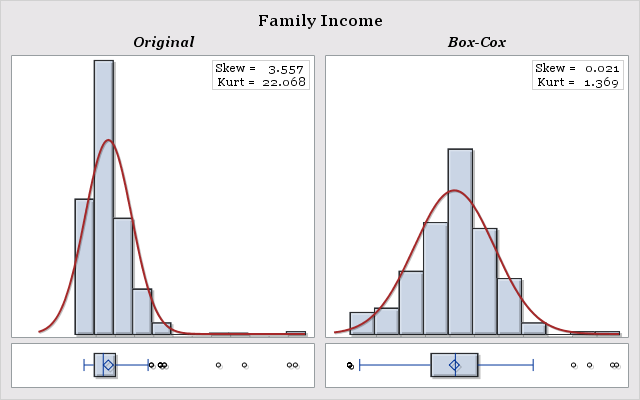
- Mark as New
- Bookmark
- Subscribe
- Mute
- RSS Feed
- Permalink
- Report Inappropriate Content
Use DYNAMICS instead of macro variables. You already have some dynamics in your template code. The assigment of the value is on the DYNAMIC statement in PROC SGRENDER (at the bottom of your code).
Hope this helps!
Dan
- Mark as New
- Bookmark
- Subscribe
- Mute
- RSS Feed
- Permalink
- Report Inappropriate Content
That gets me part of the way there. But, I now have to pass the values to proc sgrender. So, I am thinking that I need to wrap a macro around this proc. That still leaves the question of how to automate the values of skewness and kurtosis in macro variables in an automated fashion. My goal is to call up a macro procedure and only pass the dataset name and variables. I want SAS to figure out the skewness and kurtosis and pass them on to this procedure. Is there a quick way of doing this?
Cristian
proc sgrender data=WORK._TRANSFORMED_ template=ComparativeHistograms;
dynamic _Title_='Family Income'
_Raw_ ="FAMINC" _T_ ="'T_FAMINC'n"
_Raw2_="FAMINC" _T2_="'T_FAMINC'n"
_skew1=" 3.557" _kurt1="22.068"
_skew2=" 0.021" _kurt2="1.369" ;
run;
- Mark as New
- Bookmark
- Subscribe
- Mute
- RSS Feed
- Permalink
- Report Inappropriate Content
Just provide the macro value to the dynamic in the "Dynamic" statement in the SGRENDER procedure.
proc sgrender data=WORK._TRANSFORMED_ template=ComparativeHistograms;
dynamic _Title_='Family Income'
_Raw_ ="FAMINC" _T_ ="'T_FAMINC'n"
_Raw2_="FAMINC" _T2_="'T_FAMINC'n"
_skew1="&skew1" _kurt1="&kurt1"
_skew2="&skew2" _kurt2="&kurt2" ;
run;
- Mark as New
- Bookmark
- Subscribe
- Mute
- RSS Feed
- Permalink
- Report Inappropriate Content
So close. I was able to generate the exact figures that I want. However, I am having a bit of trouble saving them. Below is the code I am using to generate the figures. Although SAS is generating the figures, they are not being saved to the location I want. Here is the warning that I am getting for the first image.
WARNING: The IMAGENAME option or the output name contains invalid characters. H__Projects_VAM_SAS_Figures_AGE will be used as the image name prefix.
NOTE: Writing HTML Body file: sashtml22.htm
The file should have been saved in: "H:\Projects\VAM\SAS\Figures\SOL". I tried to hard code this instead of using macros but the same warning was generated. I followed the example in Jeff Cartier's SUGI paper but it does not seem to work for me. Any suggestions?
Cristian
%Macro ComparativeHistograms;
%do j=1 %to %sysfunc(countw(&BoxCox));
data _NULL_;
set _Moments_;
where Row=&j;
CALL SYMPUT('Raw',compress(Variable1));
CALL SYMPUT('T',compress(Variable2));
CALL SYMPUT('Lam',compress(Lambda));
CALL SYMPUT('Skew1',compress(Skew1));
CALL SYMPUT('Skew2',compress(Skew2));
CALL SYMPUT('Kurt1',compress(Kurt1));
CALL SYMPUT('Kurt2',compress(Kurt2));
run;
ods graphics on / reset imagename="&ImageLoc.\&Raw." imagefmt=png ;
proc sgrender data=WORK._TRANSFORMED_ template=ComparativeHistograms;
dynamic _Lambda="&Lam"
_Raw_ ="&Raw" _T_ ="&T"
_skew1 ="&Skew1" _kurt1 ="&Kurt1"
_skew2 ="&Skew2" _kurt2 ="&Kurt2" ;
run;
ods graphics off;
%end;
%mend;
%ComparativeHistograms;
- Mark as New
- Bookmark
- Subscribe
- Mute
- RSS Feed
- Permalink
- Report Inappropriate Content
If using LISTING destination, provide the folder name as GPATH option. Then provide the file name as you want in the IMAGENAME option on the ODS GRAPHICS statement.
Catch up on SAS Innovate 2026
Dive into keynotes, announcements and breakthroughs on demand.
Explore Now →Learn how use the CAT functions in SAS to join values from multiple variables into a single value.
Find more tutorials on the SAS Users YouTube channel.
SAS Training: Just a Click Away
Ready to level-up your skills? Choose your own adventure.


