smooth abnormalities in a time-series

[podarum]

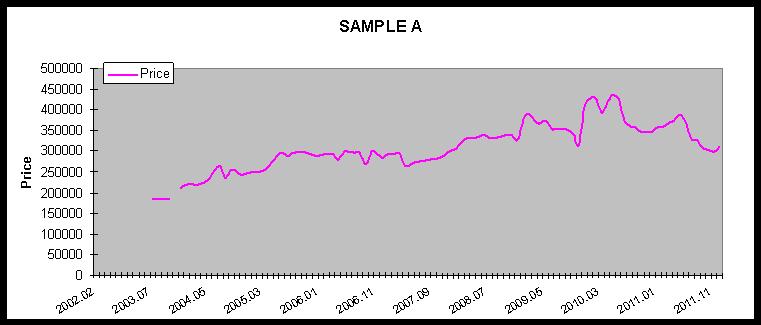
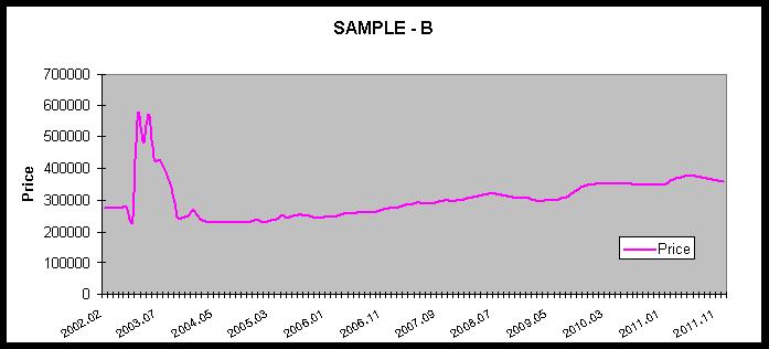
Hi,  I have many series of data (timed-series), so I'm looking for a automated procedure for this fix.  But my challenge is that I'm following a price (6-month rolling average) over a period of time that has different start dates for different series (eg. stores and products)...  and the main challenge is that I have these spikes in prices, that could happen at any point in time and for an undisclosed time-frame.  See Sample charts below.  I need to somehow smooth out these spikes, but only where they are real explosive.  So does anyone know in SAS how I can smooth out the data if for example the data has a 200% growth over a 1 year period.. but since it's gradually increasing since this is monthly data, I have to be careful I don't smooth out good data.  What I mean by that is that if the first month it increase by 20% (reasonable) and second month again another 20% (reasonable), and so on,, in one year it is 240%,.. how can I capture and smooth that.   Or I'd love to hear any other suggestions on how to deal wiht this issue.  I do have SAS/ETS.

Thanks so much.

For example I don't really want to smooth out anything in SAMPLE -A but do want the spike in SAMPLE -B

[udo_sas]

Hello -

One approach which you might want to consider is to winsorize your data using ESM for example.

Here is an example:

*create some test data by adding some extreme spike;

data air;

set sashelp.air;

if date="01JAN1954"d then air=air+200;

run;

*plot the modified series;

proc sgplot data=air;

series x=date y=air;

run;

*run ESM with WINTERS method - since the data is seasonal and trending upwards, in your case you might have to use a different technique, such as SIMPLE;

proc esm data=air out=_null_ outfor=want lead=0;

id date interval=month;

forecast air / method=winters;

run;

*replace values which have a bad fit with the ESM forecast - of course you will need to find out what flags "bad fit" in your context;

data want;

set want(rename=actual=air drop=_name_ upper lower);

if abs(error) ge 1*std and air ne 0 then air=predict;

drop error std predict;

run;

*plot the result;

proc sgplot data=want;

series x=date y=air;

run;

Instead of using the prediction of ESM you could also use other values such as the series median, or the previous value, etc.

In this case you could set the values with bad fit to missing and use TIMESERIES to replace the missing values in a 3rd step.

Hope this makes sense,

Udo

[podarum]

As usual Thanks Udo.. I will try it and post..

[podarum]

Hi Udo.. I like this approach and seems to be the right one.. but where I get stuck is where you mentioned  "of course you will need to find out what flags "bad fit" in your context;" as this is an importnat piece of the assignment.  I other words, every month is a relatively small incremental increase, which could be normal, but 4 or 5 months together could add to a abnormal spike, which is what I want to target. But can't becasue of these small monthly increases.  Know what I mean?  I'd appreciate if you have any suggestions. Of coarse you also menationed that I can set the "bad  fit" to missing and replace with timeseries, but again I don't know how to assign the bad fit definition.    Thanks Udo.

[udo_sas]

Hello -

Some additional thoughts on my response (for what it's worth):

• the first challenge I see is to identify an appropriate forecasting model, to avoid filtering out a "signal". If your data is seasonal then spikes can represent a pattern of course, if your data is trending upwards (or downwards) - as it seems to be the case - you will need to use a trend model. Maybe you will need a model which allows for both trend and seasonality. ESM provides you with access to all of these models. If you would have access to HPF as well, then your could use PROC HPF to do a best pick approach. Note the ESM models consider a local trend instead of a global trend - for a nice overview see: http://www.sas.com/reg/wp/corp/3478
• The signal to noise ratio is also important to figure out the right value for how many STD to consider. If your data is fairly noisy, then higher values of STD will make more sense, as otherwise you will be filtering data which are not really extreme values. The examples you provided seem to suggest that your data is not very noisy.
• It might also be worthwhile to consider to difference your data - so instead of the original series you will try to analyze the series of first differences. In this case you should be able to detect "huge" changes in the data even better.

Example:

data air;

set sashelp.air;

if date="01JAN1954"d then air=air+200;

air2=dif(air);

run;

proc sgplot data=air;

series x=date y=air2;

run;

Thanks,

Udo

[podarum]

Thanks Udo... i started playing with Lags and differences and am seeing couple of roadblocks in that.. for example if the data starts high and then drops 100% to a normal level, or if the data starts normal and then has a long period increase like more than 7 months, and then back to normla, I still get a spike... too many tricks to cover..

[udo_sas]

Would you be able to share some example data with me?

Thanks!

Udo

[podarum]

Data is monthly based,  on a 6-month rolling average...

All 4 samples have spikes in different ways that I'd like to get rid of..  Thanks Udo

Date           Price

2003.03      571

2003.04      483

2003.05      571

2003.06      428

2003.07      428

2003.08      395

2003.09      334

2003.10      242

2003.11      243

2003.12      251

2004.01      267

2004.02      244

... it could gradually go up to Price= 600 which is fine...

And another Sample is

Date           Price

2002.11      267

2002.12      278

2003.01      330

2003.02      390

2003.03      571

2003.04      483

2003.05      571

2003.06      428

2003.07      428

2003.08      395

2003.09      334

2003.10      242

2003.11      243

2003.12      251

2004.01      267

2004.02      244

SAMPLE 3

Date           Price

2002.11      267

2002.12      278

2003.01      330

2003.02      390

2003.03      571

2003.04      483

2003.05      571

2003.06      428

2003.07      428

2003.08      395

2003.09      334

2003.10      242

2003.11      243

2003.12      600

2004.01      644

2004.02      674

And Last sample:

Date           Price

2002.11      675

2002.12      680

2003.01      688

2003.02      290

2003.03      300

2003.04      323

2003.05      364

2003.06      375

2003.07      380

2003.08      395

2003.09      334

2003.10      242

2003.11      243

2003.12      251

2004.01      267

2004.02      244

[podarum]

To make things interesting, I also need to deal with hills... so sharp dips in the data .. exactly the same pattern, but inverted as above...

[PGStats]

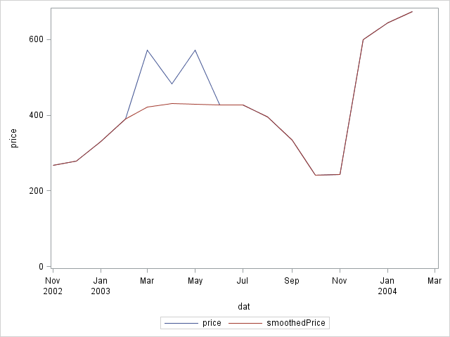
A quick intervention to mention the possible usefulness of proc convert (part of SAS ETS). If you have a means to identify the time series features that you want to smooth out then proc convert offers many interpolation methods to do the replacements. An example:

/* Use variable keep to censor the unwanted prices */

data test(drop=datxt);
input datxt $ price keep;
dat = input(compress(datxt,"."),yymmn6.);
format dat yymmP7.;
if keep then censoredPrice = price;
datalines;
2002.11      267 1
2002.12      278 1
2003.01      330 1
2003.02      390 1
2003.03      571 0
2003.04      483 0
2003.05      571 0
2003.06      428 1
2003.07      428 1
2003.08      395 1
2003.09      334 1
2003.10      242 1
2003.11      243 1
2003.12      600 1
2004.01      644 1
2004.02      674 1
;

/* Replace the unwanted prices */

proc expand data=test out=smoothTest from=month to=month;
id dat;
convert censoredPrice = smoothedPrice;
run;

PG

PG added a graph.

[podarum]

Great info .. thanks PGStats

[udo_sas]

Hello -

Many thanks for sharing your data examples. Needless to state that this is a challenging exercise, also due to the limited amount of history and the different types of "spikes".

We are currently working on a new procedure which should be useful for tackling these kind of challenges, which is not released yet. Basically it will provide access to "time series segmentation" methods, which will allow you to separate a series into a major and minor series.

As an illustration:

Unfortunately this won't help you today, as this procedure has not made its way to the production release, yet.

I thought maybe some other smoothing techniques might be useful. So I ran PROC LOESS on your data - again with mixed results, but it might give you some idea on how to proceed.

I'm not exactly an expert in using this procedure, but here it goes (I combined all your examples in one data set and used SAMPLE as a series indicator):

proc loess data=test;

   model price=dat /select=AICC;

   by sample;

run;

For the same sample as above LOESS creates the following graph:

and

so you could filter out point which have a high residual.

Unfortunately this approach does not work well if the spikes are at the beginning or end of the series.

Not sure if this is really helpful - but I thought I share it anyway.

Thanks,

Udo

[podarum]

Hi Udo,  very good to know.. For now I used a lag on Price and a lag o the lag and so on, for 4 months.. then set it to if the price drop between lags is a certain threshold OR climbs by a certain threshold, then indicate it... then use proc expand to create a moving average to smooth it out..