- Home
- /
- Programming
- /
- Programming
- /
- Capturing 95% CI Limits (so CI bands can be plotted) from PROC LIFETES...
- RSS Feed
- Mark Topic as New
- Mark Topic as Read
- Float this Topic for Current User
- Bookmark
- Subscribe
- Mute
- Printer Friendly Page
- Mark as New
- Bookmark
- Subscribe
- Mute
- RSS Feed
- Permalink
- Report Inappropriate Content
Greetings,
I am using PROC LIFETEST to calculate values for a KM plot, and then using PROC SGPLOT to plot the curves. Is there a way to use PDS OUTPUT to capture the CI band values that are shown in this plot that is output directly from LIFETEST?
Here is my code (as you can see, I've been trying to see what output dataset they might be routed to):
ods output CensoredSummary = cs
           Means           = mean
		   quartiles       = quart;

ods trace on;

proc lifetest data = acmort0 alphaqt = 0.05 plots = survival (cb atrisk = 0 to 30 by 3);
     time aval * cnsr(1);
     strata cvhgrpn / notest;
     run;
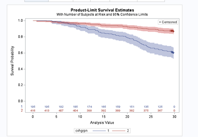
Here is the plot created by LIFETEST, which includes the confidence bands:
Is there any way to capture the band values so I can plot them myself via SGPLOT?
I realize that it's possible to customize the plot created by PROC LIFETEST (a "Warren Kuhfeld special"), but the program I inherited doesn't do it that way and I don't want to disturb it at this point in our project timeline.
Thank you!
Accepted Solutions
- Mark as New
- Bookmark
- Subscribe
- Mute
- RSS Feed
- Permalink
- Report Inappropriate Content
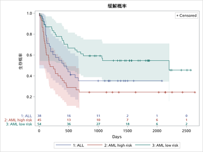
You want this ?
proc format;
   value grpLabel 1='ALL' 2='AML low risk' 3='AML high risk';
run;

data BMT;
        input DIAGNOSIS Ftime Status Gender@@;
        label Ftime="Days";
        format Diagnosis grpLabel.;
datalines;
1       2081       0       1       1       1602    0       1
1       1496       0       1       1       1462    0       0
1       1433       0       1       1       1377    0       1
1       1330       0       1       1       996     0       1
1       226        0       0       1       1199    0       1
1       1111       0       1       1       530     0       1
1       1182       0       0       1       1167    0       0
1       418        2       1       1       383     1       1
1       276        2       0       1       104     1       1
1       609        1       1       1       172     2       0
1       487        2       1       1       662     1       1
1       194        2       0       1       230     1       0
1       526        2       1       1       122     2       1
1       129        1       0       1       74      1       1
1       122        1       0       1       86      2       1
1       466        2       1       1       192     1       1
1       109        1       1       1       55      1       0
1       1          2       1       1       107     2       1
1       110        1       0       1       332     2       1
2       2569       0       1       2       2506    0       1
2       2409       0       1       2       2218    0       1
2       1857       0       0       2       1829    0       1
2       1562       0       1       2       1470    0       1
2       1363       0       1       2       1030    0       0
2       860        0       0       2       1258    0       0
2       2246       0       0       2       1870    0       0
2       1799       0       1       2       1709    0       0
2       1674       0       1       2       1568    0       1
2       1527       0       0       2       1324    0       1
2       957        0       1       2       932     0       0
2       847        0       1       2       848     0       1
2       1850       0       0       2       1843    0       0
2       1535       0       0       2       1447    0       0
2       1384       0       0       2       414     2       1
2       2204       2       0       2       1063    2       1
2       481        2       1       2       105     2       1
2       641        2       1       2       390     2       1
2       288        2       1       2       421     1       1
2       79         2       0       2       748     1       1
2       486        1       0       2       48      2       0
2       272        1       0       2       1074    2       1
2       381        1       0       2       10      2       1
2       53         2       0       2       80      2       0
2       35         2       0       2       248     1       1
2       704        2       0       2       211     1       1
2       219        1       1       2       606     1       1
3       2640       0       1       3       2430    0       1
3       2252       0       1       3       2140    0       1
3       2133       0       0       3       1238    0       1
3       1631       0       1       3       2024    0       0
3       1345       0       1       3       1136    0       1
3       845        0       0       3       422     1       0
3       162        2       1       3       84      1       0
3       100        1       1       3       2       2       1
3       47         1       1       3       242     1       1
3       456        1       1       3       268     1       0
3       318        2       0       3       32      1       1
3       467        1       0       3       47      1       1
3       390        1       1       3       183     2       0
3       105        2       1       3       115     1       0
3       164        2       0       3       93      1       0
3       120        1       0       3       80      2       1
3       677        2       1       3       64      1       0
3       168        2       0       3       74      2       0
3       16         2       0       3       157     1       0
3       625        1       0       3       48      1       0
3       273        1       1       3       63      2       1
3       76         1       1       3       113     1       0
3       363        2       1
;
run;

proc sort data=bmt;by diagnosis;run;

ods select none;
ods output SurvivalPlot=SurvivalPlot;
proc lifetest data=bmt plots=survival(cb atrisk=0 to 2500 by 500);
time ftime*Status(0);
strata diagnosis;
run;
ods select all;


title '缓解概率';
proc sgplot data=SurvivalPlot;
band x=Time lower=HW_LCL upper=HW_UCL/ group=Stratum transparency=0.8 modelname='x';
step x=Time y=Survival / group=Stratum lineattrs=(pattern=solid)  name='x' ;
scatter x=Time y=Censored / group=Stratum markerattrs=(symbol=plus) ;
xaxistable atrisk / x=tatrisk class=stratum colorgroup=stratum valueattrs=(weight=bold) location=inside;
inset '+ Censored' /position=ne border;
keylegend 'x';
run;
- Mark as New
- Bookmark
- Subscribe
- Mute
- RSS Feed
- Permalink
- Report Inappropriate Content
Hello,
See the WORK.ABC (outsurv=) dataset! ABC has columns for the confidence band.
ods graphics on;
proc lifetest data=VALung plots=(s,ls,lls) outtest=Test maxtime=600
              outsurv=ABC CONFBAND=ALL /*CONFTYPE=LOGLOG*/;
   time SurvTime*Censor(1);
   id Therapy;
   strata Cell;
   test Age Prior DiagTime Kps Treatment;
run;
ods graphics off;
Koen
- Mark as New
- Bookmark
- Subscribe
- Mute
- RSS Feed
- Permalink
- Report Inappropriate Content
What did the ODS trace output show in the log?
The plot object(s) item should be shown. ODS <nameofitem>=yourdatasetname; referencing the plot item should capture the data if CI was included in the plot. I haven't worked with lifetest but a few other procs us PLOTS as the Ods object.
There is however likely to be some manipulation of the resulting data to get it into the form that Sgplot or Sgpanel would like as there can be different types of values associated with the same x,y coordinate and you will need to reshape the data a bit.
- Mark as New
- Bookmark
- Subscribe
- Mute
- RSS Feed
- Permalink
- Report Inappropriate Content
Hello @davehalltwp ,
For what @ballardw is suggesting, you can see an example of that approach here:
https://communities.sas.com/t5/Statistical-Procedures/Proc-Gam/m-p/904749#M44902
Koen
- Mark as New
- Bookmark
- Subscribe
- Mute
- RSS Feed
- Permalink
- Report Inappropriate Content
You want this ?
proc format;
   value grpLabel 1='ALL' 2='AML low risk' 3='AML high risk';
run;

data BMT;
        input DIAGNOSIS Ftime Status Gender@@;
        label Ftime="Days";
        format Diagnosis grpLabel.;
datalines;
1       2081       0       1       1       1602    0       1
1       1496       0       1       1       1462    0       0
1       1433       0       1       1       1377    0       1
1       1330       0       1       1       996     0       1
1       226        0       0       1       1199    0       1
1       1111       0       1       1       530     0       1
1       1182       0       0       1       1167    0       0
1       418        2       1       1       383     1       1
1       276        2       0       1       104     1       1
1       609        1       1       1       172     2       0
1       487        2       1       1       662     1       1
1       194        2       0       1       230     1       0
1       526        2       1       1       122     2       1
1       129        1       0       1       74      1       1
1       122        1       0       1       86      2       1
1       466        2       1       1       192     1       1
1       109        1       1       1       55      1       0
1       1          2       1       1       107     2       1
1       110        1       0       1       332     2       1
2       2569       0       1       2       2506    0       1
2       2409       0       1       2       2218    0       1
2       1857       0       0       2       1829    0       1
2       1562       0       1       2       1470    0       1
2       1363       0       1       2       1030    0       0
2       860        0       0       2       1258    0       0
2       2246       0       0       2       1870    0       0
2       1799       0       1       2       1709    0       0
2       1674       0       1       2       1568    0       1
2       1527       0       0       2       1324    0       1
2       957        0       1       2       932     0       0
2       847        0       1       2       848     0       1
2       1850       0       0       2       1843    0       0
2       1535       0       0       2       1447    0       0
2       1384       0       0       2       414     2       1
2       2204       2       0       2       1063    2       1
2       481        2       1       2       105     2       1
2       641        2       1       2       390     2       1
2       288        2       1       2       421     1       1
2       79         2       0       2       748     1       1
2       486        1       0       2       48      2       0
2       272        1       0       2       1074    2       1
2       381        1       0       2       10      2       1
2       53         2       0       2       80      2       0
2       35         2       0       2       248     1       1
2       704        2       0       2       211     1       1
2       219        1       1       2       606     1       1
3       2640       0       1       3       2430    0       1
3       2252       0       1       3       2140    0       1
3       2133       0       0       3       1238    0       1
3       1631       0       1       3       2024    0       0
3       1345       0       1       3       1136    0       1
3       845        0       0       3       422     1       0
3       162        2       1       3       84      1       0
3       100        1       1       3       2       2       1
3       47         1       1       3       242     1       1
3       456        1       1       3       268     1       0
3       318        2       0       3       32      1       1
3       467        1       0       3       47      1       1
3       390        1       1       3       183     2       0
3       105        2       1       3       115     1       0
3       164        2       0       3       93      1       0
3       120        1       0       3       80      2       1
3       677        2       1       3       64      1       0
3       168        2       0       3       74      2       0
3       16         2       0       3       157     1       0
3       625        1       0       3       48      1       0
3       273        1       1       3       63      2       1
3       76         1       1       3       113     1       0
3       363        2       1
;
run;

proc sort data=bmt;by diagnosis;run;

ods select none;
ods output SurvivalPlot=SurvivalPlot;
proc lifetest data=bmt plots=survival(cb atrisk=0 to 2500 by 500);
time ftime*Status(0);
strata diagnosis;
run;
ods select all;


title '缓解概率';
proc sgplot data=SurvivalPlot;
band x=Time lower=HW_LCL upper=HW_UCL/ group=Stratum transparency=0.8 modelname='x';
step x=Time y=Survival / group=Stratum lineattrs=(pattern=solid)  name='x' ;
scatter x=Time y=Censored / group=Stratum markerattrs=(symbol=plus) ;
xaxistable atrisk / x=tatrisk class=stratum colorgroup=stratum valueattrs=(weight=bold) location=inside;
inset '+ Censored' /position=ne border;
keylegend 'x';
run;
- Mark as New
- Bookmark
- Subscribe
- Mute
- RSS Feed
- Permalink
- Report Inappropriate Content
Thanks everybody. I learned stuff from every response!
Catch up on SAS Innovate 2026
Dive into keynotes, announcements and breakthroughs on demand.
Explore Now →Learn how use the CAT functions in SAS to join values from multiple variables into a single value.
Find more tutorials on the SAS Users YouTube channel.
SAS Training: Just a Click Away
Ready to level-up your skills? Choose your own adventure.


