display a function

[CerditoSalvaje]

Hello everybody,

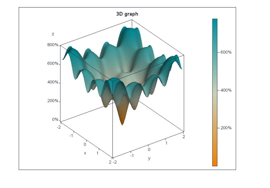
I want to display a graph with the ackley function.

/*ackley function*/
y=(-20)*(exp(-0.2*sqrt(0.5*(x[1]**2+x[2]**2))))-(exp(0.5*(cos(2*4*atan(1)*x[1])+cos(2*4*atan(1)*x[2]))))+exp(1)+20;

For this, I will use g3d, g3grid and maybe gcontour. 

The first step is to create the data statement in order to have x, y and z. 

I have : z=y*x

then the form of x and y must be similar than the form of the table sashelp.lake

But, I need x and y from an uniform law. 

I have code the beginning in IML: 

proc iml;
xmax=2;
xmin=-2;
range=xmax-xmin;
Y=j(range,1,0);
X=j(range,1,0);
X1=j(range*range,1,0);
do i=1 to range;
	call randgen(u,'uniform');
	Y[i,1]=xmin+u*range;
end;

do i=1 to range/2;
	y=y//y;
end;

do i=1 to range;
	call randgen(u1,'uniform');
	X[i,1]=xmin+u1*range;
end;

do i=1 to range;
	do n=1 to range*range;
		X1[n,1]=X[i,1];
	end;
end;
print X1;
run;
quit;

At the end, I have the correct Y but, I don't get the correct form of X which is like :

range times the first value, range times the second, etc.

Thank you for your help.

[acordes · Accepted solution]

proc iml;
_x=do(-2,2,0.05);
_y=_x;
x=expandgrid(_x,_y);

z=j(nrow(x),3,.);
do i=1 to nrow(x);
z[i,1]=(-20)*(exp(-0.2*sqrt(0.5*(x[i,1]**2+x[i,2]**2))))-
(exp(0.5*(cos(2*4*atan(1)*x[i,1])+cos(2*4*atan(1)*x[i,2]))))+exp(1)+20;
z[i,2:3]=x[i,];
end;
create in_graph from z [colname={'z' 'x' 'y'}];
append from z;
close;
run;

/* From Rick's post at:                                     */
/* http://blogs.sas.com/content/iml/create-surface-plot-sas */
proc template;                        /* surface plot with continuous color ramp */
define statgraph SurfaceTmplt;
dynamic _KMS _AGE _Z _Title;              /* dynamic variables */

 begingraph;
 entrytitle _Title;                   /* specify title at run time (optional) */
  layout overlay3d / tilt=30
          xaxisopts=(label="x")
          yaxisopts=(label="y" linearopts=(tickvaluelist=(-2 -1 0 1 2 )))
          zaxisopts=(label="z" linearopts=(tickvalueformat=xval.));
		  
  
    surfaceplotparm x=_KMS y=_AGE z=_Z /  /* specify variables at run time */

       name="surface" 
       surfacetype=fill
       colormodel=threecolorramp      /* or =twocolorramp */
       colorresponse=_Z 
       reversecolormodel=true;
    continuouslegend "surface";

    
  endlayout;
endgraph;
end;
run;

/* And... Render the Hat! */
proc sgrender data=in_graph template=SurfaceTmplt; 
   dynamic _KMS='X' _AGE='Y' _Z='Z' _Title="3D graph";
format Z percent7.1;
run;

[CerditoSalvaje]

Thank you very much. Very helpful.

[Rick_SAS]

Wow, except for vectorizing the Ackley function, these programs are virtually identical, right down to the references! I don't think I've ever seen that before for a long program.

[Rick_SAS]

If you want to create points on a uniform grid, use the EXPANDGRID function. If you want to create a surface plot, see Create a surface plot in SAS - The DO Loop

%let dx = 0.1;
%let dy = 0.1;

proc iml;
xmin=-2;
xmax=2;
xLin = do(xmin, xmax, &dx);

ymin=-2;
ymax=2;
yLin = do(ymin, ymax, &dy);

grid = expandgrid(xLin, yLin);
x = grid[,1];
y = grid[,2];

/*ackley function*/
pi = constant('pi');
z = -20*(exp(-0.2*sqrt(0.5*(x##2+y##2)))) -
        (exp(0.5*(cos(2*pi*x)+cos(2*pi*y)))) + exp(1) + 20;

create Ackley var {x y z};
append;
close;
QUIT;

title "Quick Visualization";
proc sgplot data=Ackley;
scatter x=x y=y / colorresponse=z markerattrs=(symbol=SquareFilled size=14)
                  colormodel=ThreeColorRamp;
run;

/* https://blogs.sas.com/content/iml/2015/10/12/create-surface-plot-sas.html */
proc template;                        /* surface plot with continuous color ramp */
define statgraph SurfaceTmplt;
dynamic _X _Y _Z _Title;              /* dynamic variables */
 begingraph;
 entrytitle _Title;                   /* specify title at run time (optional) */
  layout overlay3d;
    surfaceplotparm x=_X y=_Y z=_Z /  /* specify variables at run time */
       name="surface" 
       surfacetype=fill
       colormodel=threecolorramp      /* or =twocolorramp */
       colorresponse=_Z;              /* prior to 9.4m2, use SURFACECOLORGRADIENT= */
    continuouslegend "surface";
  endlayout;
endgraph;
end;
run;
proc sgrender data=Ackley template=SurfaceTmplt; 
   dynamic _X='X' _Y='Y' _Z='Z' _Title="Ackley Function";
run;

[CerditoSalvaje]

Thank you, Rick.