- RSS Feed
- Mark Topic as New
- Mark Topic as Read
- Float this Topic for Current User
- Bookmark
- Subscribe
- Mute
- Printer Friendly Page

- Mark as New
- Bookmark
- Subscribe
- Mute
- RSS Feed
- Permalink
- Report Inappropriate Content
Product and division have the same evaluation priority, without parentheses they are evaluated from left to right. Your equation is equivalent to
( (p[2]-x)*p[3]/x)*(p[4]+x)##p[5] - p[1]
It should read
(p[2]-x)*p[3]/(x*(p[4]+x)##p[5]) - p[1]
PG

- Mark as New
- Bookmark
- Subscribe
- Mute
- RSS Feed
- Permalink
- Report Inappropriate Content
I expect that you will encounter all kinds of problems like this. For the FROOT function, the INTERVAL argument is supposed to be an interval [a,b] such that f(a) and f(b) have different signs and f is continuous on [a,b].
You see the comment that says:
/* Optional: Call function that computes interval that has root */
It means that you should use knowledge of your problem to compute an interval [a,b] for each pair of parameters. For rational functions that have k branches, you need to decide which root you want.
(If the denominator of your expression has k-1 zeros, then the rational function has k branches.)

- Mark as New
- Bookmark
- Subscribe
- Mute
- RSS Feed
- Permalink
- Report Inappropriate Content
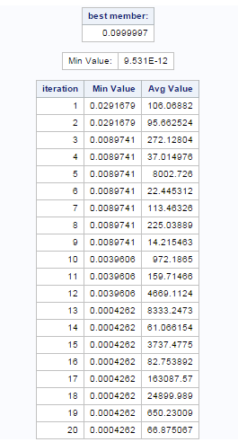
Use my GA code ![]() . Unlike FROOT() , GA don't ask for a special interval . You can define a very wide range , like me , I set it in [-10,10] .
. Unlike FROOT() , GA don't ask for a special interval . You can define a very wide range , like me , I set it in [-10,10] .
Code: Program
proc iml;
start func(x);
 v=abs(  (0.3-x)*2/(x*(1+x)**2) - 3.3058  );
 return (v);
finish;

id=gasetup(1,1,1234);
call gasetobj(id,0,"func");
call gasetsel(id,100,1,0.95);
call gasetcro(id,0.4,4);
call gasetmut(id,0.4);

call gainit(id,10000,{-10,10});
niter = 100;
summary = j(niter,2);
mattrib summary [c = {"Min Value", "Avg Value"} l=""];
do i = 1 to niter;
 call garegen(id);
 call gagetval(value, id);
 summary[i,1] = value[1];
 summary[i,2] = value[:];
end;
call gagetmem(mem, value, id, 1);
print mem[ l="best member:"],
   "Min Value: " value[l = ""] ;
iteration = t(1:niter);
print iteration summary;
call gaend(id);
quit;
Xia Keshan
- Mark as New
- Bookmark
- Subscribe
- Mute
- RSS Feed
- Permalink
- Report Inappropriate Content
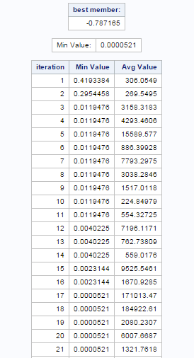
How about using Genetic Algorithms ? which can be used under the situation that function is not differentiable or continuous .
And you define a width range of interval to search root . Unlike Rick and PG need to define a very good start point .
I love GA a hell of a lot .
Code: Program
proc iml;

start func(x);
 v=abs((0.3-x)*2/(1+x)**2 - 48);
 return (v);
finish;

id=gasetup(1,1,1234);
call gasetobj(id,0,"func");
call gasetsel(id,100,1,0.95);
call gasetcro(id,0.4,4);
call gasetmut(id,0.4);

call gainit(id,10000,{-10,10});
niter = 100;
summary = j(niter,2);
mattrib summary [c = {"Min Value", "Avg Value"} l=""];
do i = 1 to niter;
 call garegen(id);
 call gagetval(value, id);
 summary[i,1] = value[1];
 summary[i,2] = value[:];
end;
call gagetmem(mem, value, id, 1);
print mem[ l="best member:"],
   "Min Value: " value[l = ""] ;
iteration = t(1:niter);
print iteration summary;
call gaend(id);
quit;
Xia Keshan
- Mark as New
- Bookmark
- Subscribe
- Mute
- RSS Feed
- Permalink
- Report Inappropriate Content
An interesting alternative is to hijack the machinery of proc nlin with a single observation. The specification of starting values is very flexible in proc nlin.
/* Equation has the form p1 = (p2-x)*p3/(p4+x)**p5 */
data parms;
eqNo + 1;
input p1-p5;
datalines;
48 0.3 2 1 2
25 0.1 4 1 2
;
data startingValues;
set parms;
parameter = "x";
do Estimate = -0.95*p4 to -0.05*sign(p4) by 0.05*sign(p4);
output;
end;
keep eqNo parameter Estimate;
run;
proc nlin data=parms noprint outest=roots(where=(_TYPE_="FINAL"));
by eqNo;
parameters / pdata=startingValues;
model p1 = (p2-x)*p3/(p4+x)**p5;
run;
proc print data=roots noobs;
var EqNo _STATUS_ _SSE_ x;
format x best12.;
run;
PG

- Mark as New
- Bookmark
- Subscribe
- Mute
- RSS Feed
- Permalink
- Report Inappropriate Content
Hello PG,
Thank you your help.
It seems that in your program there is no solution when you have x in the denominator. For instance if you change the equation to
model p1 = (p2-x)*p3/(x*(p4+x)**p5); and the datelines to
3.3058 0.3 2 1 2
The solution should be 0.1
May be that your program does not converge because the function has a discontinuity at x=0. If you can restrict the solution to be in the interval (0.01 , 1) - where the solutions should fall in my work computing cost of capital for firms, which cannot be negative and very unlikely to exceed 100% .
Can your program restrict the analysis to this interval ( 0.01,1) so a solution is obtained? .
One more question, if you do not mind, is whether your program can provide the different solutions (assuming that they are several positive solutions less than 1).
Thank you again
- Mark as New
- Bookmark
- Subscribe
- Mute
- RSS Feed
- Permalink
- Report Inappropriate Content
Hi Thomas,
As long as you know an interval where the root is, an interval that doesn't include a singularity (re 's comments), you should be able to find the root. For example, if such an interval is (0.01, 1) for equation 3.4 = (0.3-x)*2/(x*(1+x)**2), the root will be found by:
data parms;
eqNo + 1;
input p1-p5;
datalines;
3.4 0.3 2 1 2
;
data startingValues;
set parms;
parameter = "x";
do Estimate = 0.01 to 1.00 by 0.05; /* Scan the root interval */
output;
end;
keep eqNo parameter Estimate;
run;
proc nlin data=parms outest=roots(where=(_TYPE_="FINAL"));
by eqNo;
parameters / pdata=startingValues;
model p1 = (p2-x)*p3/(x*(p4+x)**p5);
run;
proc print data=roots noobs;
var EqNo _STATUS_ _SSE_ x;
format x best12.;
run;
PG
- Mark as New
- Bookmark
- Subscribe
- Mute
- RSS Feed
- Permalink
- Report Inappropriate Content
Thank you again PG,
The program works, but I wonder if you know why the program gives me outcomes outside (0,1) so the
do Estimate = 0.01 to 1.00 by 0.05; /* Scan the root interval */
does not seem to exclude negative and/or > 1 roots.
One example:
data parms;
eqNo + 1;
input p1-p26;
datalines;
0 3.797547029 4.367179084 3.8961265 3.425073916 2.954021332 2.482968748 2.011916165 1.540863581
1.069810997 0.598758413 0.127705829 12.83196748 12.83196748 12.83196748 12.83196748 12.83196748
12.83196748 12.83196748 12.83196748 12.83196748 12.83196748 12.83196748 12.83196748 12.83196748 11.96
;
data startingValues;
set parms;
parameter = "x";
do Estimate = 0.01 to 1.00 by 0.05; /* Scan the root interval */
output;
end;
keep eqNo parameter Estimate;
run;
proc nlin data=parms outest=roots(where=(_TYPE_="FINAL"));
by eqNo;
parameters / pdata=startingValues;
model p26 =
p13+(p13*(p1-x)/(1+x)**1)+(p14*(p2-x)/(1+x)**2)+ (p15*(p3-x)/(1+x)**3)+
(p16*(p4-x)/(1+x)**4)+ (p17*(p5-x)/(1+x)**5)+ (p18*(p6-x)/(1+x)**6)+
(p19*(p7-x)/(1+x)**7)+ (p20*(p8-x)/(1+x)**8)+ (p21*(p9-x)/(1+x)**9)+
(p22*(p10-x)/(1+x)**10)+ (p23*(p11-x)/(1+x)**11)+ (p24*(p12-x)/(1+x)**12)+
(p25*(p12-x)/(x*(1+x)**12));
run;
proc print data=roots noobs;
var EqNo _STATUS_ _SSE_ x;
format x best12.;
run;
- Mark as New
- Bookmark
- Subscribe
- Mute
- RSS Feed
- Permalink
- Report Inappropriate Content
Yes, x is unbounded. The startingValues dataset contains a list of possible starting values for NLIN. The function is evaluated for every starting value and the best one is kept. From there, the optimisation algorithm will move x until it finds the root or until a maximum number of iterations is reached.
You can force some hard bounds on x with a BOUNDS statement in NLIN :
BOUNDS 0.01 <= x <= 1;
PG

- Mark as New
- Bookmark
- Subscribe
- Mute
- RSS Feed
- Permalink
- Report Inappropriate Content
The right-hand-side of the 2 examples is the ratio of 1 polynomial over another polynomial.
You write: "the actual polynomial have 12 terms". Do both polynomials (numerator and denominator) have 12 terms? Or does the equation have a grand total of 12 parameters?
- Mark as New
- Bookmark
- Subscribe
- Mute
- RSS Feed
- Permalink
- Report Inappropriate Content
A pedestrian view of the question.
The function (F) in question has 26 parameters and thus a clear view is complicated.
The function (F) has poles at x=0 and x=-1 so the roots of F will not include 0 and -1.
First, assign some values to the said 26 parameters.
Second, find at least 1 root of F within either in the (0 to 1) or (0 to -1) range.
Assumption about the parameters:
1- p13 and p26 are greater than 1, with p26> p13.
2- besides p13 and p26, the other parameters are positive and less than 1.
I am using a crude and pedestrian method to find the roots.
/************************************************/
/**** sample random sets of parameters p(26) ****/
/************************************************/
data t_a(keep=i p:);
array p(26);
do i = 1 to 10;
do j = 1 to 26;
if (j=13) then p(j)= ceil(30*ranuni(5));
else if (j=26) then p(j)= p(13)+ ceil(20*ranuni(7));
else p(j) = ceil(10000*ranuni(11))/10000;
end;
output;
end;
run;
/************************************************/
/**** for each set of parameters find a root ****/
/************************************************/
data t_b(keep=i p: aZero aChng aRoot bSign);
array p(26);
set t_a;
aSign=0;
aZero=0;
aFunc=0;
aChng=0;
aSteps=1000;
bSign=1;
do j=0 to aSteps;
aZero=bSign*j*(1/aSteps);
aFlag=aFunc;
do k=1 to 14;
if (k=1) then aFunc+(p(13)-p(26))*aZero*((1+aZero)**12);
else if (k=14) then aFunc+(p(25)*(p(12)-aZero));
else aFunc+(p(11+k)*(p(k-1)-aZero)*aZero*((1+aZero)**(13-k)));
end;
aFunc= round(aFunc,0.00001);
if (j=0) then aSign= sign(aFunc);
else if not(sign(aFunc)=aSign) then do;
aChng=1;
aRoot= aZero-bSign*(1/aSteps)*(abs(aFunc)/(abs(aFunc)+abs(aFlag)));
aRoot=round(aRoot,0.000001);
leave;
end;
end;
output;
run;
proc print data=t_b;
var i bSign aZero aRoot aChng;
format aRoot 9.6;
run;
/********************/
/*** some results ***/
/********************/
When looking at the (0 to 1) range (bSign=1) one finds at least 1 root (aRoot).
aChng=1 -> the function (aFunc) changed signs.
i bSign aZero aRoot aChng
===================================
1 1 0.059 0.058985 1
2 1 0.431 0.430937 1
3 1 0.024 0.023931 1
4 1 0.007 0.006165 1
5 1 0.024 0.023457 1
6 1 0.012 0.011116 1
7 1 0.014 0.01384 1
8 1 0.127 0.126725 1
9 1 0.108 0.107417 1
10 1 0.025 0.024228 1
When looking at the (0 to -1) range (bSign=-1), not all sets of p(26) have a
root in the (0 to -1) range. No root (aRoot=.) when there is no change in sign (aChng=0).
i bSign aZero aRoot aChng
======================================
1 -1 -1 . 0
2 -1 -0.057 -0.056783 1
3 -1 -0.144 -0.143403 1
4 -1 -1 . 0
5 -1 -0.256 -0.255269 1
6 -1 -0.056 -0.055367 1
7 -1 -1 . 0
8 -1 -0.416 -0.415036 1
9 -1 -0.042 -0.041868 1
10 -1 -0.279 -0.278255 1
- « Previous
-
- 1
- 2
- Next »
.jpg")
Catch up on SAS Innovate 2026
Nearly 200 sessions are now available on demand in the Innovate Hub.
Watch Now →- Ask the Expert: Fast, Clear, Beautiful: Your First Steps With PROC SGPLOT | 04-Jun-2026
- Ask the Expert: R and SAS Working Seamlessly Together: Unlocking PROC R in Viya for Life Sciences | 11-Jun-2026
- Ask the Expert: Can Agents Reduce Planning Friction in CPG Supply Chains? | 16-Jun-2026
- Ask the Expert: Get Meaningful Results With New Features in SAS Customer Intelligence 360 | 25-Jun-2026
-
25 replies
-
06-11-2015 12:52 PM
-
7102 views
-
7 likes
-
5 in conversation
-
