Next-Generation Data Mining and Machine Learning: Python and SAS® Together at Last

[#1]

Paper 1051-2021

Authors

 George S. Habek, M.S., CT Global Solutions, Inc.; Suman Kumar Das, CT Global Solutions, Inc.

Abstract

Have you developed Python models to solve a business problem and want to use them in a next-generation analytical framework? Learn how to use Python to create a bridge between open source and SAS Visual Data Mining and Machine Learning, which is automated, dynamic and scalable. Compete and compare next-generation algorithms to select a champion seamlessly. The business problem will be within the transportation shipping industry. A variety of data elements (such as internal factors of package size, delivery day of the week, number of transit days; external factors of weather and financial effects) will also be used. The ultimate business questions are: What is the best subset of factors that drive cost? What is the optimal model to use to score a new prospect file with the predicted average cost? Discover how Python and SAS Visual Data Mining and Machine Learning can work together to answer these critical questions for the shipping company.

Watch the presentation

Watch Next-Generation Data Mining and Machine Learning: Python and SAS® Together at Last by the author on the SAS Users YouTube channel.

Introduction

The world has been severely impacted by COVID-19.  As a result, many organizations are facing unprecedented challenges.  Specifically, the transportation shipping industry, needs to qualify the factors causing fluctuations of its shipping cost across their networks.  Given the possible complexity of various networks, the desire to have a comprehensive data mining & machine learning platform has become mission critical.  Due to the numerous possible causal factors within the industry, ensuring the “best” algorithm is utilized to determine the most important factors driving costs is at the forefront of the organization’s needs. 

Why is this so important?  The transportation company ultimately desires to be profitable across all their customers.  Therefore, establishing the most important causal factors driving shipping cost enables the company to better price the various package shipments across the network for the customers.  This creates actionable business results optimizing profitability among customers.

Available Data

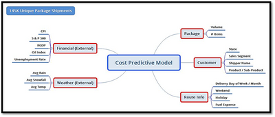
A variety of factors (external and internal) are available for the analysis.  Figure 1 illustrates the different attributes.  First, approximately 145K unique package shipments were utilized in the model development.  External factors pertaining to financial information such as CPI and Unemployment Rate were used.  In addition, external factors related to weather such as average rainfall and temperature were used.  Internal factors pertaining package, customer, and route information were also utilized.

Figure 1. Available Data

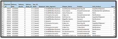
Below is a sample of the raw data used in the analysis.

Figure 2A. Sample Data

Figure 2B. Sample Data

Open-Source Connection – Install & Configure Python 2.7.x or 3.4+

There are steps required for installing and configuring the Python version utilized.  First, Python should be installed in the Compute server of the SAS Viya environment.  Next, the executable file must be available in the system path in the SAS Compute server.  The system path is in “opt/sas/viya/config/etc/sysconfig/compsrv/default/sas-compsrv” on compute server.  To connect to python from SAS VDMML, the environment variable needs to be set as “export PATH=path_to_your_python_bin_directory:${PATH}” in the sas-compsrv file.  The final step is to provide sudo privileges to the python packages so that other users can access all the Python libraries/packages.

The following is a snippet of sas-compsrv file with Python path variable.

 

Figure 3. sas-compsrv file

Develop Python Models Via Jupyter Notebook

Python is one of the leading open-source programming languages. Integrating Python with a state-of-the-art data mining & machine learning environment – SAS® VDMML will help solve the business problem stated earlier. First, let us discuss the native Python models in the Jupiter notebook.

Scikit-learn (Sklearn) is a very popular library for machine learning techniques in Python. Sklearn has many useful machine learning models and efficient statistical methods. In this paper, we will be using this library for different analysis in native Python and then integrate models within SAS. There are many features of the Sklearn library, including Clustering, Ensemble Methods, Supervised Models, Cross-Validation (estimation of the accuracy of supervised models on new data), etc.…

In this section, we are going to cover 4 different supervised models in native Python.

• Linear Regression with Elastic Net
• Neural Network using Multi-layer Perceptron (MLP)
• Decision Tree
• Random Forest

Linear Regression with Elastic Net

For linear regression, we are using the Elastic Net regularized regression method which combines L1 and L2 penalties. You can control these penalties separately also.

The following table illustrates the basic parameters for the Elastic Net regression method.

Parameter name	Description
Alpha	Constant that multiplies the penalty terms. Default value is 1.0.
L1_Ratio	This ratio defines how L1 and L2 parameter applied. Default value is 0.5. For l1_ratio = 0 the penalty is an L2 penalty. For l1_ratio = 1 it is an L1 penalty. For 0 < l1_ratio < 1, the penalty is a combination of L1 and L2.
Fit_Intercept	Default value is True means Data is not centered.
Normalize	Default value is True which means regressors X will be normalized before regression by subtracting the mean and dividing by the l2-norm.
Warm_Start	Default value is True. When set to True, reuse the solution of the previous call to fit as initialization, otherwise, just erase the previous solution
Selection	Default value is ‘cycle’. If set to ‘random’, a random coefficient is updated every iteration rather than looping over features sequentially by default.

 Table 1. Basic parameters for Linear Regression with Elastic Net

Before we start building the model, there are always data preparation steps required which includes cleaning the data, removing unwanted variables, removing variables that show multicollinearity, encoding categorical string values to numeric value, etc...

#Changing the Categorical string values to numerical value before build the model
from sklearn.metrics import r2_score, mean_squared_error
from sklearn.preprocessing import LabelEncoder
lencoders = {}
for col in proc_data.select_dtypes(include=['object']).columns:
	lencoders[col] = LabelEncoder()
	proc_data[col] = lencoders[col].fit_transform(proc_data[col])

#dropping the Shipment_Expense variable from input variables
X=proc_data.drop('shipping_expense', axis=1)

#Setting the target variable for the model
Y=proc_data['shipping_expense']

#Splitting the data for train the model and validate
from sklearn.model_selection import train_test_split
x_train, x_val, y_train, y_val=train_test_split(X,Y,test_size=0.10,random_state=12345)
#Changing the Categorical string values to numerical value before build the model
from sklearn.metrics import r2_score, mean_squared_error
from sklearn.preprocessing import LabelEncoder
lencoders = {}
for col in proc_data.select_dtypes(include=['object']).columns:
	lencoders[col] = LabelEncoder()
	proc_data[col] = lencoders[col].fit_transform(proc_data[col])

#dropping the Shipment_Expense variable from input variables
X=proc_data.drop('shipping_expense', axis=1)

#Setting the target variable for the model
Y=proc_data['shipping_expense']

#Splitting the data for train the model and validate
from sklearn.model_selection import train_test_split
x_train, x_val, y_train, y_val=train_test_split(X,Y,test_size=0.10,random_state=12345)

 Figure 4.  Python Overall Data Preparation

Now the data is ready for the supervised models. We build the Linear Regression model penalized with Elastic Net (L1: 50% and L2: 50%) in Jupiter notebook. When predicting the value, the validation dataset will be used. The validation data set is created in the data preparation step. Model comparison will happen based on the Root Mean Square Error (RMSE).  The model with the smallest RMSE will be deemed the champion.

#Parameters for the Linear Regression Model using ElasticNet. L1_ratio 0.5 means L1=50 and L2=50
#All other parameters will have default values.
params_lr={'l1_ratio':0.5}

#Build the linear regression model with Elastic Net
from sklearn.linear_model import ElasticNet
model_lr=ElasticNet(**params_lr)
model_lr.fit(x_train,y_train)

#Prediction on the validation data
pred_train_enet=model_lr.predict(x_val)

#Calculate the Mean Squared Error and display the root Mean Squared Error value
mse=mean_squared_error(y_val,pred_train_enet)
print("Root Average Squared Error = {}".format(math.sqrt(mse)))

Figure 5.  Python Linear Regression Model using Elastic Net

 

Neural Network using Multi-layer Perceptron (MLP)

After we build one of the simple supervised models, i.e., linear regression, we are now ready to build a series of linear regression iterations, which is called a neural network model. A Multi-layer Perceptron (MLP) regressor is used for the neural network Model. Advantages of using MPL regressors are the following:

• Capability to learn non-linear models
• Capability to learn models in real-time (on-line learning).
• Supports multi output regression so that the sample can have more than one target.

MLP has different layers:

• Input Layer - Input variables or visible layer
• Hidden Layers – Layers of different nodes between input layer and output layer.
• Output Layers – This Layer represents the output variables

The following table illustrates the basic parameters for the Neural Network MLP algorithm.

Parameter Name	Description
Hidden_Layer_Sizes	Default value is (100,). The ith element represents the number of neurons in the ith hidden layer.
Activation	Default value is ‘relu’. Activation function for the hidden layer. ·         ‘identity’, no-op activation, useful to implement linear bottleneck, returns f(x) = x ·         ‘logistic’, the logistic sigmoid function, returns f(x) = 1 / (1 + exp(-x)). ·         ‘tanh’, the hyperbolic tan function, returns f(x) = tanh(x). ·         ‘relu’, the rectified linear unit function, returns f(x) = max(0, x)
Solver	Default value is ‘adam’. This value used for weight optimization. Default value works very well on large datasets in terms of training time and validation score. ·         ‘lbfgs’ is an optimizer in the family of quasi-Newton methods. ·         ‘sgd’ refers to stochastic gradient descent. ·         ‘adam’ refers to a stochastic gradient-based optimizer
Alpha	Default value is 0.0001. L2 penalty parameter.
Max_Iter	Default value is 200. Maximum number of iterations. The solver iterates until convergence (determined by ‘tol’) or this number of iterations. For stochastic solvers (‘sgd’, ‘adam’), note that this determines the number of epochs (how many times each data point will be used), not the number of gradient steps.

Table 2. Basic parameters for Neural Network with MLP

For the MLP regressor parameters, 3 hidden layers are modelled here, with 30 neurons in each layer. Therefore, there are total of 5 layers including the input and output layers. We are using the ‘lbfgs’ optimizer which works best when you have limited memory. It stores only the last few updates to save memory. In addition, activation is ‘relu’ (rectified linear activation function) which uses a linear function for output but in fact, a non-linear function allows complex modelling in the hidden layers. With this activation, it is easier to train the model and achieve better performance. Also, maximum iteration is 500 for this model to run until it converges.

#Parameters for the Neural Network Model with MLP regressor
params = {'hidden_layer_sizes': (30,30,30), 'activation': 'relu', 'solver': 'lbfgs', 'max_iter': 500}

#Build the MLP Regressor model
from sklearn.neural_network import MLPRegressor
model_lr = MLPRegressor(**params)
model_lr.fit(x_train,y_train)


#Prediction on the validation data
pred_train_enet=model_lr.predict(x_val)

#Calculate the Mean Squared Error and display the root Mean Squared Error value
mse=mean_squared_error(y_val,pred_train_enet)
print("Root Average Squared Error = {}".format(math.sqrt(mse)))

 Figure 6.  Python Neural Network model using MLP

Decision Tree

 The decision tree algorithm is one of the most popular models in supervised learning, because it is very easy to explain.  The decision tree algorithm uses if-else conditions and splits the data into multiple segments. The algorithm selects the optimal number of splits. The goal of the algorithm is to ask questions on the data while narrowing the possible values within each split until the model achieves confidence to make a prediction.  

The following table illustrates a sample of the basic parameters for the Decision Tree algorithm used.

Parameter Name	Description
Criterion	The function to measure the quality of split. Possible options are – ·         ‘mse’, - mean squared error ·         ‘friedman_mse’ – mean squared error with Friedman’s improvement score for potential splits ·         ‘mae’ – mean absolute error. ·         ‘Poisson’ – uses reduction in Poisson deviance to find splits.
Splitter	The strategy uses to choose the split at each node in the tree. Default option is ‘best’. Options are ‘best’ and ‘random’.
Max_Depth	The maximum depth of the tree.
Max_Features	The number of features to consider when looking for the best split.

Table 3. Basic parameters for the Decision Tree algorithm

In the Decision Tree model, we have considered the ‘friedman_mse’ function as the criterion to split the data. Also, the splitter = ‘best’ option is used so that the algorithm will take the feature with the highest importance instead of randomness. The maximum feature for our model is ‘sqrt’ which means sqrt(n_features) where n_features is the number of features when the model fit is performed.

#Parameters for the Decision Tree Model
params = {'criterion': "friedman_mse", 'splitter': "best", 'max_depth': 16, 'max_features': "sqrt"}

#Build the Decision Tree Regressor model
from sklearn.tree import DecisionTreeRegressor
model_lr = DecisionTreeRegressor(**params)
model_lr.fit(x_train,y_train)

#Prediction on the validation data
pred_train_enet=model_lr.predict(x_val)

#Calculate the Mean Squared Error and display the root Mean Squared Error value
mse=mean_squared_error(y_val,pred_train_enet)
print("Root Average Squared Error = {}".format(math.sqrt(mse)))

 Figure 7.  Python Decision Tree algorithm

Random Forest

After the decision tree model is developed, we can extend that tree and build a series of decision trees, which is called a Random Forest model. The random forest algorithm creates random samples of the data, and then the algorithm creates a separate tree for each sample.  Finally, the model prediction is created by taking the average of each tree to improve model accuracy and control over-fitting. 

The following table illustrates the basic parameters for the Random Forest algorithm.

Parameter Name	Description
N_Estimators	The number of trees in the forest.
Criterion	The function to measure the quality of a split. Supported criteria are “mse” for the mean squared error, which is equal to variance reduction as feature selection criterion, and “mae” for the mean absolute error.
Max_Depth	The maximum depth of the tree.
Min_Samples_Split	The minimum number of samples required to split an internal node.
Min_Samples_Leaf	The minimum number of samples required to be at a leaf node.

Table 4. Basic parameters for Random Forest algorithm

The following parameters were utilized for the random forest algorithm:

• Maximum depth of the tree equal to 20.
• Minimum samples required to split at any leaf equal to 5.
• Total number of trees in the forest is 100.
• All other parameters are set to default.

#Parameters for the Random Forest Regressor Model
params = {'n_estimators': 100, 'max_depth': 20, 'min_samples_leaf': 5}

#Build the Random Forest Regressor model
from sklearn.ensemble import RandomForestRegressor
model_lr = RandomForestRegressor(**params)
model_lr.fit(x_train,y_train)

#Prediction on the validation data
pred_train_enet=model_lr.predict(x_val)

#Calculate the Mean Squared Error and display the root Mean Squared Error value
mse=mean_squared_error(y_val,pred_train_enet)
print("Root Average Squared Error = {}".format(math.sqrt(mse)))

 Figure 8.  Python Random Forest algorithm

Now that four Python models have been developed, it makes sense to compare them and select a champion.  The random forest algorithm was deemed to be the champion model based on the Root Mean Square Error (RMSE), which provided the smallest value across the four models.

Incorporate Python Models Within SAS VDMML Pipeline

We will now shift our focus to a state-of-the-art data mining & machine learning environment – SAS® VDMML.  This platform resides on VIYA, which is a cloud-enabled, in-memory analytics engine that provides a dynamic, automated, and scalable insights, leading to actionable business results.  Before we begin incorporating Python and SAS® VDMML, we need to discuss the metadata for the business problem outlined earlier.  If you recall, the business challenge is to establish the causal factors that drives the shipping expense for each package shipment across the logistics transportation network.  There are three basic layers of the metadata that needs to be assigned:

• Target – This is what we are trying to predict (Y or Response) – in our example it is Shipping_Expense
• Inputs – These are the independent factors (X’s) – which includes attributes around external information like weather and financial data, as well as internal information related to the logistics organization.  This is referenced in Figure 1 in the paper earlier.
• Rejected – These are factors that will not be used in the analysis, as they are either not related to the business problem or are highly influential to the Target.

Next, we will introduce the concept of a pipeline, where the data mining & machine learning will be executed.  Since we must compare Python & SAS models, there are 8 total algorithms that will be assessed.  Therefore, two pipelines were created for ease of use.  Let us discuss the first pipeline.  Before, we start applying the models, it is a best practice to explore the data.  There are some analytical preparation tasks that are usually done prior to model development.  For example, inspection for variable skewness, which indicates the need for possible transformations; another task is inspection for missing data, which indicates the need for possible imputations.  In our analysis, there was no need to apply any transformations or imputations to the data.

In the first pipeline, we will discuss Linear Regression & Decision Tree models for Python & SAS.  To include the SAS models, you select Supervised Learning Models from the Data node.  Then, you select Linear Regression & Decision Tree models, respectively.  There are several options to select for each model setting.  We will review some basic ones.  For Linear Regression, there are three options utilized:

• Stepwise – This uses a hybrid approach of forward and backward selection, which has been proven to be powerful in establishing significant factors driving the response (Shipping_Expense).
• Adjusted R-Square – This is the statistic utilized to select the final subset of factors, which accounts for the factors introduced in the model, and measures the amount of true variability being explained with respect to the Target.
• Model interpretability using variable importance – This illustrates the final set of factors ordered from the most to least significant in predicting the Target.

Now, we will discuss the Python models for the first pipeline.  To include open-source code within the pipeline, you need to select “Add child node” >> “Miscellaneous” >> “Open-Source Code”.  The next step is to choose what type of open-source code is desired.  In our example, we will select Python.  Please make sure to select the “Use output data in child nodes” option, otherwise, the data will not be passed to any other following nodes in the pipeline, such as scoring, if that is desired.  By default, this option is not selected.

  Figure 9.  Python Node Properties

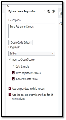
The final step is to insert the Python Linear Regression model, which we have developed in the previous section, by clicking on the Open Code Editor button. Before we use the Python code, let us review some of the key terms that will be used within the Python open-source code.

• dm_input – The list which represents the input variables (interval and categorical).
• dm_partitionvar – The String variable, identifies the name of the data partition. Values can be 1, 0 and 2 for training, validation, and test, respectively.
• dm_partition_train_val – This variable contains the value of the data partition for training set. The value is 1.
• dm_inputdf – This is a data frame which represents sample input data observations.
• dm_dec_target – This is the target variable in this case ‘Shipping_Expense’
• dm_traindf – This is a data frame which holds a sample training data.
• dm_nodedir – This variable contains node’s working directory.

All these variables are set by SAS VDMML based on the data and selection options we chose. We fit the model based on the training partition data. This has been accomplished by adding the ‘fullX_enc[dm_partitionvar] == dm_partition_train_val’ code. If desired to use the validation data instead for the model, then the code can be replaced by ‘fullX_enc[dm_partitionvar] == dm_partition_valid_val’. Finally, the model predicted the average ‘Shipping Expense’ on the complete input data.

We have used the same parameters and algorithms that we have used in native Python to build the model. All the Python code from SAS VDMML will be passed to the Python environment and executed from there, and the result returned to SAS VDMML to display the variable importance, plots, files, and any of the result tables.

When the output results or files created are stored in the ‘dm_nodedir’ location, then those fields can be displayed in the result pane. We are displaying the variable importance files to the result window.

The following is the Python Linear Regression model code.

import sys
#Linear Regression by Elasticnet
from sklearn.linear_model import ElasticNet

#Partition The Data
dm_input.insert(0, dm_partitionvar)
fullX = dm_inputdf.loc[:, dm_input]
fullX_enc = pd.get_dummies(fullX, columns=dm_class_input, drop_first=True)
X_enc = fullX_enc[fullX_enc[dm_partitionvar] == dm_partition_train_val]
X_enc = X_enc.drop(dm_partitionvar, 1)
y = dm_traindf[dm_dec_target]

#Build the Model
dm_model = ElasticNet()
dm_model.fit(X_enc, y)
print(dm_model)

#Display the Variable Importance
varimp = pd.DataFrame(list(zip(X_enc, dm_model.coef_)), columns=['Variable Name', 'Importance'])
varimp.to_csv(dm_nodedir + '/rpt_var_imp.csv', index=False)

fullX_enc = fullX_enc.drop(dm_partitionvar, 1)
#Prediction On The Validation Data
dm_scoreddf = pd.DataFrame(dm_model.predict(fullX_enc), columns=['P_shipping_expense'])

Figure 10.  Python Linear Regression Model Code in SAS VDMML

Now, we are ready to discuss the SAS Decision Tree model.  There are some basic options utilized:

• Splitting – The default settings are fine; however, the Minimum Leaf Size is set to 30 instead of 5, which allows for the smallest number of training observations that a leaf can have.  This value is a recommended best practice to ensure enough data exists for the splitting process.
• Pruning – The default settings are fine.
• Model interpretability using variable importance – This illustrates the final set of factors ordered from the most to least significant in predicting the Target.

Next, we will add another open-source node for the Python Decision Tree model, similarly to the Python Linear Regression model discussed previously in this section.  The following figure is the Python Decision Tree model with all the same parameters that have been used in native Python. Also, the partition logic for the decision tree model uses the same code as the Linear Regression model open-source code.

#Decision Tree Model
from sklearn.tree import DecisionTreeRegressor

#Partition The Data
dm_input.insert(0, dm_partitionvar)
fullX = dm_inputdf.loc[:, dm_input]
fullX_enc = pd.get_dummies(fullX, columns=dm_class_input, drop_first=True)
X_enc = fullX_enc[fullX_enc[dm_partitionvar] == dm_partition_train_val]
X_enc = X_enc.drop(dm_partitionvar, 1)
y = dm_traindf[dm_dec_target]

#Build The Model
params = {'criterion': "friedman_mse", 'splitter': "best", 'max_depth': 16, 'max_features': "sqrt"}
dm_model = DecisionTreeRegressor(**params)
dm_model.fit(X_enc, y)
print(dm_model)

#Display the Variable Importance
varimp = pd.DataFrame(list(zip(X_enc, dm_model.feature_importances_)), columns=['Variable Name', 'Importance'])
varimp.to_csv(dm_nodedir + '/rpt_var_imp.csv', index=False)

fullX_enc = fullX_enc.drop(dm_partitionvar, 1)
#Predict On the Validation Data
dm_scoreddf = pd.DataFrame(dm_model.predict(fullX_enc), columns=['P_shipping_expense'])

Figure 11.  Python Decision Tree Model Code in SAS VDMML

The following figure illustrates the finished Pipeline 1 diagram.

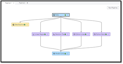
Figure 12.  SAS® VDMML Pipeline 1

After Pipeline 1 has been run, the model comparison node displays that SAS VDMML Linear Regression is the wining model with 18.27 for the Root Average Squared Error (RASE).  The champion model was selected due to having the lowest value for RASE.  Although there are many options to choose for model comparison, best practice suggests using the RASE, as it is an absolute measure of fit.  It is a good measure of how accurately the model predicts the response (Shipping_Expense), and it is the most important criterion for fit if the main purpose of the model is prediction.

Figure 13.  SAS® VDMML Pipeline 1 Model Comparison

Let us now proceed to Pipeline 2.  In the second pipeline, we will discuss Neural Network & Random Forest models for Python & SAS.  To include the SAS models, you select Supervised Learning Models from the Data node.  Then, you select Neural Network & Random Forest models, respectively.  There are several options to select for each model setting.  We will review some basic ones.  For the Neural Network model, we will use the default settings with one minor change: Model interpretability using variable importance – This illustrates the final set of factors ordered from the most to least significant in predicting the Target.

Next, we will add another open-source node for the Python Neural Network model, similarly to the other Python models already discussed in the previous section.  The following figure is the Python Neural Network model code with all the same parameters that have been used in native Python. Also, the partition logic for the Neural Network model uses the same code as for the previous Python code.

import sys
#Neural Network-MLPRegressor
from sklearn.neural_network import MLPRegressor

#Partition The Data
dm_input.insert(0, dm_partitionvar)
fullX = dm_inputdf.loc[:, dm_input]
fullX_enc = pd.get_dummies(fullX, columns=dm_class_input, drop_first=True)
X_enc = fullX_enc[fullX_enc[dm_partitionvar] == dm_partition_train_val]
X_enc = X_enc.drop(dm_partitionvar, 1)
y = dm_traindf[dm_dec_target]

#Build The Model
params = {'hidden_layer_sizes': (30,30,30), 'activation': 'relu', 'solver': 'lbfgs', 'max_iter': 500}
dm_model = MLPRegressor(**params)
dm_model.fit(X_enc, y)
print(dm_model)

#Prediction On the Validation Data
fullX_enc = fullX_enc.drop(dm_partitionvar, 1)
dm_scoreddf = pd.DataFrame(dm_model.predict(fullX_enc), columns=['P_shipping_expense'])

Figure 14.  Python Neural Network Model Code in SAS VDMML

Now, we are ready to discuss the SAS Random Forest model.  The default settings including building 100 trees within the forest and one minor change: Model interpretability using variable importance – This illustrates the final set of factors ordered from the most to least significant in predicting the Target.

Next, we will add another open-source node for the Python Random Forest model, similarly to the other Python models already discussed in the previous section.  The following figure is the Python Random Forest model code with all the same parameters that have been used in native Python. Also, the partition logic for the Random Forest model uses the same code as for the previous Python code.

import sys
#Random Forest Model
from sklearn.ensemble import RandomForestRegressor

#Partition The Data
dm_input.insert(0, dm_partitionvar)
fullX = dm_inputdf.loc[:, dm_input]
fullX_enc = pd.get_dummies(fullX, columns=dm_class_input, drop_first=True)
X_enc = fullX_enc[fullX_enc[dm_partitionvar] == dm_partition_train_val]
X_enc = X_enc.drop(dm_partitionvar, 1)
y = dm_traindf[dm_dec_target]

#Build the Model
params = {'n_estimators': 100, 'max_depth': 20, 'min_samples_leaf': 5}
dm_model = RandomForestRegressor(**params)
dm_model.fit(X_enc, y)
print(dm_model)

#Prediction On the Validation Data
fullX_enc = fullX_enc.drop(dm_partitionvar, 1)
dm_scoreddf = pd.DataFrame(dm_model.predict(fullX_enc), columns=['P_shipping_expense'])

Figure 15.  Python Random Forest Model Code in SAS VDMML

The following figure illustrates the finished Pipeline 2 diagram.

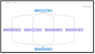
Figure 16.  SAS® VDMML Pipeline 2

After Pipeline 2 has been run, the model comparison node displays that the Python Random Forest is the winning model with approximately 17.3 for the Root Average Squared Error (RMSE).  The champion model was selected due to having the lowest value for RMSE. This analysis resembles the same conclusion that we have seen in the previous section that the Python Random Forest model was the champion.

Figure 17.  SAS® VDMML Pipeline 2 Model Comparison

Now, we need to compare all models across both pipelines.  Based on the Average Squared Error (ASE), it is evident that the final champion model has been deemed to be the Python Random Forest model, which has the lowest ASE value.

Figure 18.  SAS® VDMML Overall Pipeline Model Comparison

Finally, it is important to assess what the significant factors are from the champion model as it pertains to driving the shipping expense for the transportation logistics organization.  The figure below illustrates the factors.  For example, the most important variable is the fuel expense, which makes sense since the package shipments are delivered by vehicles.  Other important factors include the product (type of shipment), delivery time in days, shipper name (customer), average number of items for each package shipment, etc.  It is interesting to note that all the important factors related to internal data elements. 

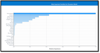
Figure 19.  SAS® VDMML Overall Model Champion – Python Random Forest Significant Factors Driving Shipping Expense

Model Deployment – Scoring Prospect File Using Champion Model

In this section, the focus will shift to applying the champion model to score a new prospect file to predict the average shipping expense for each package shipment.  If you recall, the overall champion model was deemed to be the Python Random Forest model from Pipeline 2.  The next step is to include a Score Data Node to Pipeline 2 underneath the champion model.

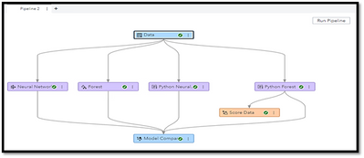
Figure 20.  SAS® VDMML Model Deployment Via Scoring

An important aspect in the model scoring & deployment process is to carefully assess how accurate the model’s predictions are.  In this example, the predictions were compared to actual shipping expenses for new prospects across the transportation network hierarchy.

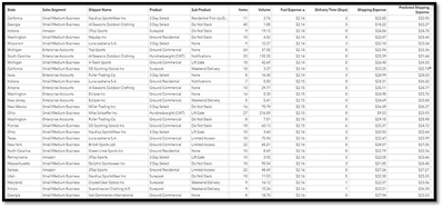
Figure 21.  SAS® VDMML Model Scoring – Actual VS. Predicted Shipping Expense

The figure above illustrates the model’s prediction is very close to the actual values of shipping expense.  For a better visualization of this, let us view the graphs below.

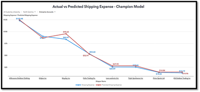
Figure 22A.  Model Scoring Visualization – Actual VS. Predicted Shipping Expense

The above visualization illustrates a slice of the complete scoring data within the transportation network hierarchy.  For example, we selected the state of North Carolina, the sales segment of Enterprise Accounts.  You can observe for the various customers, the actual and predicted shipping expense values are very close.  We can further dive deeper into the hierarchy and observe a specific customer, illustrated in the following figure.

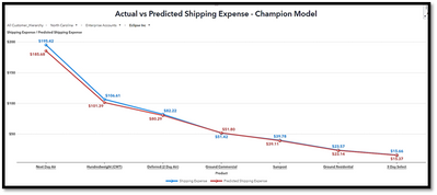
Figure 22B.  Model Scoring Visualization – Actual VS. Predicted Shipping Expense

The figure above illustrates the specific customer of “Eclipse Inc” across the various product types used for the package shipments.  Again, observe the actual and predicted shipping expense values are extremely close.  The two preceding illustrations clearly show the very good accuracy of the model.

Conclusion – Summary & Recommendations

In this paper, we have outlined a shipping organization’s critical need to determine the causal factors for the cost of package shipments across the transportation network.  Especially during this Covid disrupted world, being proactive instead of reactive towards pricing package shipments has become a necessary analytic endeavor.  Understanding these significant causal factors helps the company to establish pricing for their customers to become more profitable and brings business value in terms of scenario analysis and dynamic pricing.

Furthermore, assessing specific characteristics of these factors and how they affect the shipping expense fluctuation (+/-), has proven to be extremely valuable to the organization.

Integrating open-source models using Python, within a next generation data mining & machine learning environment, allowed for a very comprehensive analysis to address the critical business need.  The transportation shipping industry can be rather complex within the network, so the need to have state of the art analytics, leaving no stone unturned, has provided actionable business results.

Furthermore, it is a best practice to always revisit the data elements to assess if other possible factors can be introduced to enhance the modeling process.  Therefore, it would be a good exercise to investigate if other data attributes can be captured relevant to package shipments.

Finally, another valuable exercise would be to inject the shipping expense causal factors from the champion ML & AI model revealed in this discussion into a time series forecast – projecting the shipping expense for a specific time in the future.  From a best practice perspective, this has proven to substantially increase the forecast accuracy!

References

Python Open-source Model guide. Available at https://scikit-learn.org/stable/

SAS Developer Home page for all integration with Open source. Available at https://developer.sas.com/home.html.

Jagruti Kanjia and Dominique Latour, Jesse Luebbert (2020). “Using Python with Model Studio for SAS® Visual Data Mining and Machine Learning.” In Proceedings of the SAS Global Forum 2020 Conference. Cary, NC: SAS Institute Inc. Available at https://www.sas.com/content/dam/SAS/support/en/sas-global-forum-proceedings/2020/4384-2020.pdf.

June 2020. SAS^® Visual Data Mining and Machine Learning 8.5: User’s Guide

SAS Institute Inc., NC.

 

Acknowledgements

Our thanks for the excellent feedback and suggestions from the following:

• Dr. Manash R. Ray, Co-Founder & CEO, CT Global Solutions, Inc.
• Marie Tchebanenko, Presenter Coordinator, AG2R La Mondiale Group
• James R. Wolcott, Director of Operations, CT Global Solutions, Inc.