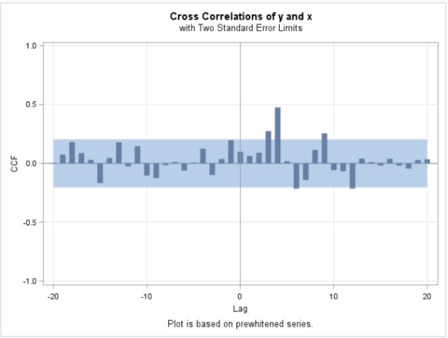
I am having difficulty coming up with the transfer model inputs. Below is the code that I have so far
proc arima data = sales plot(unpack); identify var = x noprint; estimate q = 2 noprint; identify var = y crosscorr=(x) nlag = 20; /*estimate input = (3$(2)/(1,1)x) noint printall altparm backlim = -3 plot;*/ /*estimate input = (3$(2)/(2)x) noint printall altparm backlim = -3 plot;*/ estimate input = (3$(1)/(1,2)x) noint printall altparm backlim = -3 plot; run; quit;
My question is how to come up with numerator and denominators based on the graph and differencing. I know b = 3$ since it is the number of periods it takes before xt affects yt
For s and r , I am confused:
s is from my understanding the number of lags that reside between the first spike and the beginning of the clear dying down pattern
since I have x and y with no differencing and I set s arbitrarily to s = 2 would I write input = 3$(1,2)/(1,2)
r is from my understanding 1 if the lags die down exponentially after the spikes or 2 if they down in a sine wave
since I have x and y with no differencing and since from the graph r = 2 would I input in SAS input = 3$(1,2)/(1,2)
I am confused on what specifically (1,2) means: does it mean first order differencing and r/s being chose at 2 or does 1,2 mean how many lags before there is a spike
If anyone can help me interpret my graph I would greatly appreciate it .
Thank you
Deciding the form of a transfer function relationship is explained in a book by Pankratz, A. (1991). Forecasting with Dynamic Regression Models. New York: John Wiley & Sons. Also see Pankratz, A. (1983). Forecasting with Univariate Box-Jenkins Models: Concepts and Cases. New York: John Wiley & Sons. You can also check out professor Hyndman's blog on time series analysis: https://robjhyndman.com/hyndsight/arimax/
Hope this helps.
SAS Innovate 2025 is scheduled for May 6-9 in Orlando, FL. Sign up to be first to learn about the agenda and registration!
Learn how to run multiple linear regression models with and without interactions, presented by SAS user Alex Chaplin.
Find more tutorials on the SAS Users YouTube channel.