- Home
- /
- Analytics
- /
- Forecasting
- /
- Re: Choosing between and evaluating ARIMA / ESM / UCM for a model with...
- RSS Feed
- Mark Topic as New
- Mark Topic as Read
- Float this Topic for Current User
- Bookmark
- Subscribe
- Mute
- Printer Friendly Page
- Mark as New
- Bookmark
- Subscribe
- Mute
- RSS Feed
- Permalink
- Report Inappropriate Content
My problem is outlined as follows:
I have a time series which I am trying to forecast (let's call this series OUTPUT), let's say through the end of 2018. The seasonal aspect of this value may be present, but if it is, is VERY slight. I also have two other time series (let's call them INPUT1 and INPUT2) that are being used to predict the OUTPUT series. I have values for these two series through the end of 2018 and would like to use their relationship with the OUTPUT in my forecast.
My attempts thus far have been using PROC ARIMA with an estimate statement that looks something like:
estimate p=1 input=( / (1) INPUT1 / (1) INPUT2)
But I'm unsure if this is correct. I've been unable to find any documentation anywhere on how to determine the proper differentiation or format of the inputs to use in a PROC ARIMA. It's also possible that PROC ESM or USM are more useful for this and I've been neglecting them. Any insight on how to choose and fit a forecasting model for a time series with inputs would be great. Thanks in advance.
Accepted Solutions
- Mark as New
- Bookmark
- Subscribe
- Mute
- RSS Feed
- Permalink
- Report Inappropriate Content
When doing forecasting for a time series with inputs there are several things you need to be aware of:
* Trend and seasonal components should be removed before investigating the relationship between the inputs and the target (Apply differencing to reduce the target to a stationary time series)
generate an ACF and PACF to determine trend and seasonality
proc arima data=input plots=all;
   /* t is a date variable going from 1 to N */
   identify var = target nlag=12 crosscorr=(t);
   estimate input=(t) plot ml;
run;
determine a possible AR lag from this and rerun the code with new options (let's say you determined a p=1)
proc arima data=input plots=all;
   identify var=target;
   estimate p=1 method=ml plot;
   forecast lead=12 id=t interval=month out=out1;
quit;
You've determined you have a trend, look for seasonality and difference accordingly.
proc arima data=input plots=all;
/* adf=3 if you have trend, =2 if no trend but mean different than 0, =1 if no trend and mean=0 */
 identify var=target stationarity=(adf=(3));
quit;
If we need to difference we do:
proc arima data=input plots=all;
   identify var=target(1) nlag=12;
 quit;
* Correlation between the inputs at different lags is possible (dealt with in the CCF plot). Correlation between inputs at same lags is done in 2 ways: PROC REG or PROC AUTOREG.
Using PROC REG and VIF statistic:
proc reg data=input outest=est;
   model target = input1 input2 input3 input4 /vif aic sbc;
quit;
If there are inputs with VIF>10 it means those inputs are correlated. You could try to include them in the model one at a time. Let's say input3 and input4 both have a VIF>100. Modelling both separetely would be:
ods output ParameterEstimates=parest FitStatistics=fitstat;
proc reg data=input outest=est;
   input3: model target=input1 input2 input3 / aic sbc edf dwprob;
   input4: model target=input1 input2 input4 / aic sbc edf dwprob;
   omit_var1andvar2: test input1=0, input2=0;
quit;
ods output close;
Look at a) VIF values, b) the durbin watson probabilities which tells you if a series is white noise c) significance of inputs based on their p-values.
The PROC AUTOREG solution would be:
proc autoreg data=input;
   model target = input1 input2 input3 input4 /nlag=10 backstep;
   test input1=0, input2=0;
run;
Adjust the model so that only the important variables remain and rerun proc autoreg. This will help you identify the AR part of your model.
* Autocorrelation for Input variables is possible. (Prewhiten the stationary residuals of the target and those of the inputs: PROC ARIMA a second IDENTIFY statement)
Here is an example of how to do it plus details:
* Outliers present for different inputs
If you have outliers in your data PROC ARIMA, more specifically the OUTLIER statement can help you. OR you could create a dummy variable for that input that would take the value of 1 if it's an outlier or 0 for normal values. You then use that dummy var as a separate input.
* Cross-correlate the white noise input residuals with the prewhitened target residuals and use CCF plot to identify the transfer function for the input). The target variable can be influenced by past values of the inputs (use CCF plot to determine the lags)
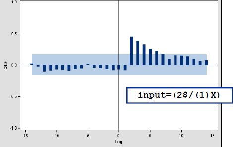
In order to make an idea of what model would fit you need to do a Cross Correlation Function. A CCF plot looks like this:
Whenever the bars pass the blue line, you record significant spikes in the data. If spikes occur at negative lags it means the target depends on future values for that input (they might be erroneous, if not use PROC VARMAX which adapts to more general models).
In this graph there are spikes at lags 1, 2, 4, 5, 10. It means the target depends on that input at those lags. Include one lag at a time in the model, not all of them at once since spikes at higher lags might be the consequence of spikes at lower lags.
Example of code on how to calculate CCF:
ods graphics on;
proc arima data=input plots=all;
  identify var=Target(1 12)
           cross=( Input1(1 12) Input2(1 12) Dummyvar1 Dummyvar2)
           nlags=12;
run;
quit;
ods graphics off;
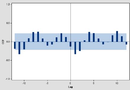
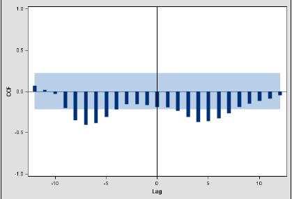
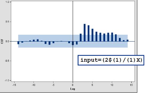
This syntax removes trend and seasonality. I've specified seasonality at lag 12, but you adapt it to what you have. If you don't remove trend and seasonality, your CCF plot would look like this:
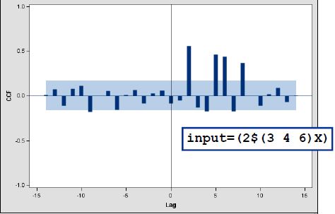
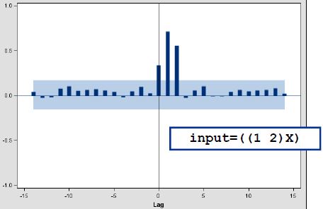
At this point you can still have correlated inputs at different lags. The CCF would give you an indication of this and you would have to determine the decay and lag factors. You will have to read about transfer functions to understand how to interpret it.
Examples of CCF:
* Diagnose an ARMA(p,q) model
The target variable can be influenced by past values of the inputs (use CCF plot to determine the lags)
proc arima data=input;
   identify var=target cross=(input1 input2 Dummyvar1 Dummyvar2) nlags=12;
   estimate p=1 input=( (1) input1 3$ input2 /1 Dummyvar1  (1) Dummyvar2) method=ml;
run;
I strongly recommend that you take the SAS course Forecasting using Base SAS, A Programming Approach. All of this and more are explained.
- Mark as New
- Bookmark
- Subscribe
- Mute
- RSS Feed
- Permalink
- Report Inappropriate Content
Hello -
ARIMA documentation provides some information on how to deal with inputs here: https://support.sas.com/documentation/cdl/en/etsug/68148/HTML/default/viewer.htm#etsug_arima_getting...
Alternatively you may want to explore UCM - which will give you the benefit of being able to explain the impact of your inputs in a more straightforward manner than ARIMAX. See https://support.sas.com/documentation/cdl/en/etsug/68148/HTML/default/viewer.htm#etsug_ucm_examples0... as an example.
ESM does not allow for inputs currently - we are working on this functionality, stay tuned.
Thanks,
Udo
- Mark as New
- Bookmark
- Subscribe
- Mute
- RSS Feed
- Permalink
- Report Inappropriate Content
When doing forecasting for a time series with inputs there are several things you need to be aware of:
* Trend and seasonal components should be removed before investigating the relationship between the inputs and the target (Apply differencing to reduce the target to a stationary time series)
generate an ACF and PACF to determine trend and seasonality
proc arima data=input plots=all;
   /* t is a date variable going from 1 to N */
   identify var = target nlag=12 crosscorr=(t);
   estimate input=(t) plot ml;
run;
determine a possible AR lag from this and rerun the code with new options (let's say you determined a p=1)
proc arima data=input plots=all;
   identify var=target;
   estimate p=1 method=ml plot;
   forecast lead=12 id=t interval=month out=out1;
quit;
You've determined you have a trend, look for seasonality and difference accordingly.
proc arima data=input plots=all;
/* adf=3 if you have trend, =2 if no trend but mean different than 0, =1 if no trend and mean=0 */
 identify var=target stationarity=(adf=(3));
quit;
If we need to difference we do:
proc arima data=input plots=all;
   identify var=target(1) nlag=12;
 quit;
* Correlation between the inputs at different lags is possible (dealt with in the CCF plot). Correlation between inputs at same lags is done in 2 ways: PROC REG or PROC AUTOREG.
Using PROC REG and VIF statistic:
proc reg data=input outest=est;
   model target = input1 input2 input3 input4 /vif aic sbc;
quit;
If there are inputs with VIF>10 it means those inputs are correlated. You could try to include them in the model one at a time. Let's say input3 and input4 both have a VIF>100. Modelling both separetely would be:
ods output ParameterEstimates=parest FitStatistics=fitstat;
proc reg data=input outest=est;
   input3: model target=input1 input2 input3 / aic sbc edf dwprob;
   input4: model target=input1 input2 input4 / aic sbc edf dwprob;
   omit_var1andvar2: test input1=0, input2=0;
quit;
ods output close;
Look at a) VIF values, b) the durbin watson probabilities which tells you if a series is white noise c) significance of inputs based on their p-values.
The PROC AUTOREG solution would be:
proc autoreg data=input;
   model target = input1 input2 input3 input4 /nlag=10 backstep;
   test input1=0, input2=0;
run;
Adjust the model so that only the important variables remain and rerun proc autoreg. This will help you identify the AR part of your model.
* Autocorrelation for Input variables is possible. (Prewhiten the stationary residuals of the target and those of the inputs: PROC ARIMA a second IDENTIFY statement)
Here is an example of how to do it plus details:
* Outliers present for different inputs
If you have outliers in your data PROC ARIMA, more specifically the OUTLIER statement can help you. OR you could create a dummy variable for that input that would take the value of 1 if it's an outlier or 0 for normal values. You then use that dummy var as a separate input.
* Cross-correlate the white noise input residuals with the prewhitened target residuals and use CCF plot to identify the transfer function for the input). The target variable can be influenced by past values of the inputs (use CCF plot to determine the lags)
In order to make an idea of what model would fit you need to do a Cross Correlation Function. A CCF plot looks like this:
Whenever the bars pass the blue line, you record significant spikes in the data. If spikes occur at negative lags it means the target depends on future values for that input (they might be erroneous, if not use PROC VARMAX which adapts to more general models).
In this graph there are spikes at lags 1, 2, 4, 5, 10. It means the target depends on that input at those lags. Include one lag at a time in the model, not all of them at once since spikes at higher lags might be the consequence of spikes at lower lags.
Example of code on how to calculate CCF:
ods graphics on;
proc arima data=input plots=all;
  identify var=Target(1 12)
           cross=( Input1(1 12) Input2(1 12) Dummyvar1 Dummyvar2)
           nlags=12;
run;
quit;
ods graphics off;
This syntax removes trend and seasonality. I've specified seasonality at lag 12, but you adapt it to what you have. If you don't remove trend and seasonality, your CCF plot would look like this:
At this point you can still have correlated inputs at different lags. The CCF would give you an indication of this and you would have to determine the decay and lag factors. You will have to read about transfer functions to understand how to interpret it.
Examples of CCF:
* Diagnose an ARMA(p,q) model
The target variable can be influenced by past values of the inputs (use CCF plot to determine the lags)
proc arima data=input;
   identify var=target cross=(input1 input2 Dummyvar1 Dummyvar2) nlags=12;
   estimate p=1 input=( (1) input1 3$ input2 /1 Dummyvar1  (1) Dummyvar2) method=ml;
run;
I strongly recommend that you take the SAS course Forecasting using Base SAS, A Programming Approach. All of this and more are explained.
April 27 – 30 | Gaylord Texan | Grapevine, Texas
Registration is open
Walk in ready to learn. Walk out ready to deliver. This is the data and AI conference you can't afford to miss.
Register now and lock in 2025 pricing—just $495!
- Ask the Expert: Wie kann ich Visual Studio Code als SAS Entwicklungsumgebung nutzen? | 11-Dec-2025
- DCSUG Online Winter Webinar | 11-Dec-2025
- Ask the Expert: Marketing Decisions Excellence: Turning Insights Into Business Impact | 16-Dec-2025
- SAS Bowl LVII, SAS Data Maker and Synthetic Data | 17-Dec-2025
- SAS Innovate 2026 | Grapevine, Texas | 27-Apr-2026

