Writing a Pluggable Modeling Strategy for SAS® Visual Forecasting

2 Likes

SAS® Visual Forecasting

SAS® Visual Forecasting (VF) is the next generation forecasting product from SAS®. It includes a web-based user interface for creating and running projects to generate forecasts from historical data. SAS® Visual Forecasting provides automation and analytical sophistication to generate millions of forecasts in the turnaround time that is necessary to run your business. Forecasters can create projects using visual flow diagrams, or pipelines, running multiple models on the same data set and choosing a champion model based on the results.

SAS® Visual Forecasting is built on SAS® Viya®, an analytic platform powered by Cloud Analytic Services (CAS). As a result, it is designed to effectively model and forecast time series on a large scale with its highly parallel and distributed architecture. This essentially provides a platform for the speed and scalability needed to create the models and generate forecasts for millions of time series. Massive parallel processing within a distributed architecture is one of the key advantages in SAS® Visual Forecasting for large scale time series forecasting.

You can generate forecasts by using the modeling strategies that are shipped with SAS® Visual Forecasting. The included modeling strategies are hierarchical forecasting, auto-forecasting, and naïve model forecasting strategies. Furthermore, you can create your own modeling strategies, and the custom strategies can be shared with other projects and forecasters. These custom modeling strategies are referred to as pluggable modeling strategies. SAS® Visual Forecasting is shipped with a pluggable hierarchical forecasting model as an illustration of its flexibility and extensibility.

How to Write a Pluggable Modeling Strategy?

The following three files are required to define a pluggable modeling strategy:

json: the metadata about the strategy
xml: the validation rules for the strategy specification settings (properties)
sas: the run-time SAS® code

These three files are packed in a zip file for uploading or downloading to and from SAS® Visual Forecasting toolbox.

Details of template.json

The template.json contains the metadata about the strategy in JSON format. The following types of information are included:

Name, description, revision, and version
Prototype, including name, revision, version, executionProviderId, status, and componentProperties containing the specifications and the corresponding default values
applicationId: Specify the application, can be either “forecasting”, “text”, or “datamining”. You should always set to “forecasting” for VF strategies
classification: set to “pluggable”
providerId: set to “CustomTemplate”
group: set to “modeling”
hidden: set to false

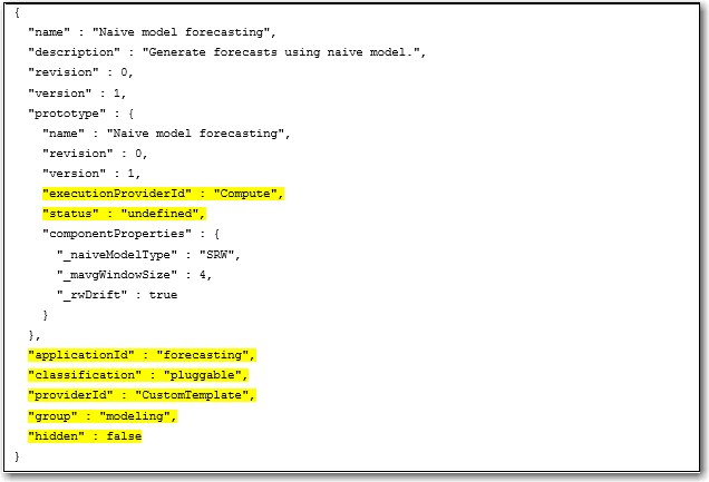
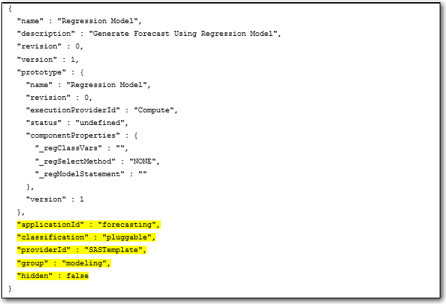
Example:

Notice that there are two copies of name, version and revision inside and outside the definition of prototype. Just remember to make sure that these two copies share the same values.

You should always set the highlighted components to have the same values as shown in the example above.

Details of validation.xml file

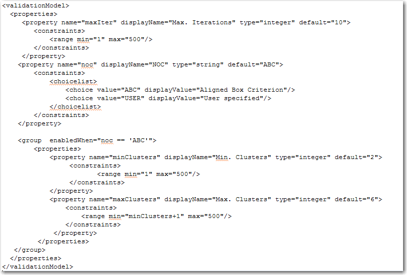
The validation.xml file validates the specification settings against valid values in XML format. The file conforms to an XML schema which is used to validate any XML you provide to the validation service when defining a new validation model. A validation model can be best described via an example:

The root element - validationModel - can have an id and a description. When used in the context of the validation service, all models are assigned an id.

Within the model a set of properties are defined within a “properties” element, which can contain any number of “property” elements, or “group” elements. Each property defined in the model describes how values are interpreted by the validation engine when it is asked to validate a map of name/value pairs. The basic required information for a property is:

name - this corresponds to the key used in the map under validation.
displayName - a localizable, user-friendly name for the property. This is provided so that a UI can query the validation model and render a control for this property.
type - the value type for this property. Currently supported types are string, integer, double and boolean.
default - (optional) a default value. When validating a map that does not contain a value for a given property, the default, if specified, is used instead.
required - (optional) true or false - indicates if a value for this property is required. The default is true.
enabledWhen (optional) - a boolean expression, which, when evaluated, indicates if this property is enabled. A property that is not enabled is not validated. This field can also be used by a UI to gray out/disable controls associated with properties that have become disabled as values in the properties map change.

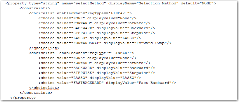
Properties can have one or more constraints. Typically, only one constraint is needed. There are two types of constraints currently supported: choice lists and ranges. You can see how these work by just referring to the example above. Constraints themselves support the “enabledWhen” attribute, so that it is possible for a property to have different constraints depending on some condition. For example, you can have a property defined as follows:

Notice the difference in the last choice value in each of the two choice lists. Here, the set of choices depend on if the property “regType” has been set to “LINEAR”.

Ranges let you specify bounds in terms of values held by other properties. For example, in this construct:

The range constraint for the second property says that value for “maxClusters” should always be at least one greater than that of “minClusters”.

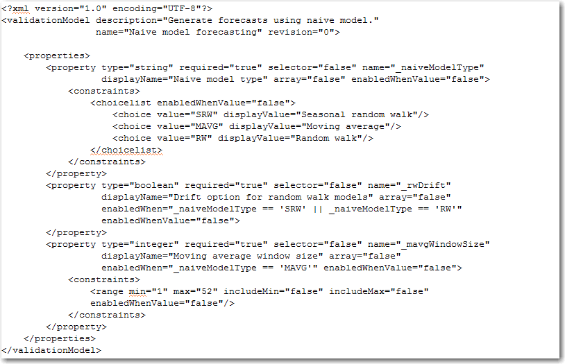
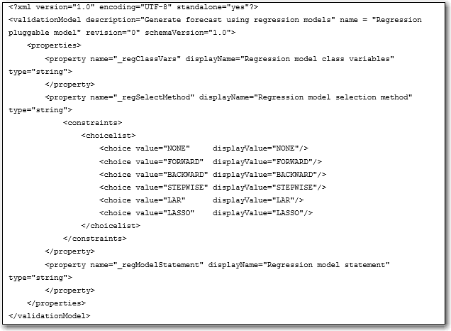
A validation.xml file example

When a pluggable modeling strategy is added to a pipeline, the strategy specifications (type, name, displayValue, choicelist, etc.) are retrieved from validation.xml file, and are displayed in the right panel with the default values defined in the template.json file and the allowable values defined in the validation.xml. See the following example for the validation.xml file associated with naïve model.

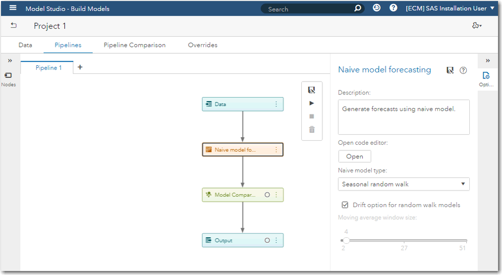
The screenshot below shows how the specifications are displayed in a pipeline.

Users can change the specification settings in the right panel. The values are saved to macro variables named using the property name defined in the validation.xml. In the above example, three macro variables are generated. It is recommended to have the property names starting with “_” so that they will not conflict with system generated macro variables.

Details of code.sas file

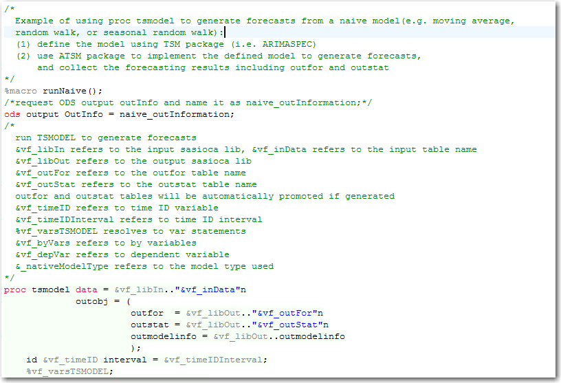
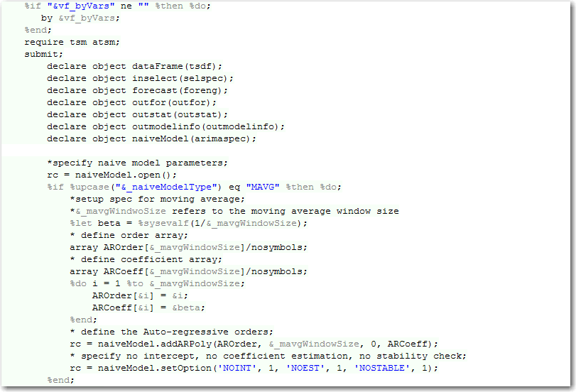
The code.sas file contains the runtime SAS® code that can be executed in a pipeline to generate forecasts. There are a set of system-defined macro variables and macros that you can use in the runtime code to obtain references to the input data, variable roles and settings, etc. from the pipeline, and references to the locations and the tables to store the resulting forecasts.

System-defined macro variables and macros

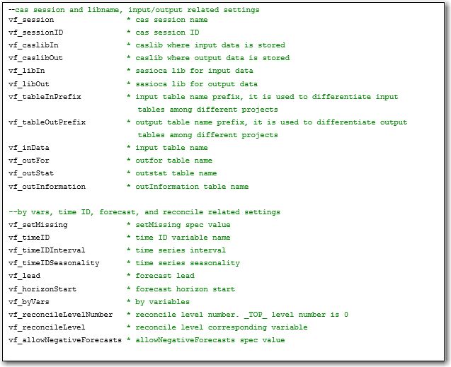
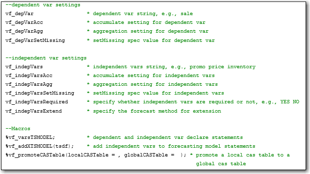
The following are the system-defined macro variables and macros containing project information such as CAS session, CASLIBS, table names, and variable roles and settings. You can refer to these macro variables and macros to retrieve information and generate PROC TSMODEL statements when writing the runtime code.

Macro vf_varsTSMODEL generates the VAR statements of the PROC TSMODEL to define the dependent and independent variables. The statements also include the acc= and setmiss= settings for the corresponding variables. For example:

Macro vf_addXTSMODEL generates addX function call of the TSDF object (from the ATSM package) for all the independent variables. For example:

You need to use the macro vf_promoteCASTable to promote any table other than the system-defined output tables if you would like to persist them for further use.

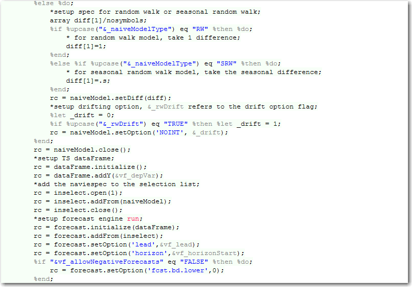
code.sas file example:

Input and Output Table Contracts

Input table contracts

The input table is prepared by the Data node in the pipeline. Please refer to the VF documentation Chapter “Setting up your project” for more information about the input data.

Output table contracts

The standard modeling node output tables are:

OUTFOR table. It contains forecasts from the forecast models. It is a required output table.

Required columns:

byVars
timeID
actual (actual value of dependent variable)
predict (predicted value of dependent variable)

Optional columns:

std (standard deviation of errors)
lower (lower confidence limit of predicted values)
upper (upper confidence limit of predicted values)

The system automatically validates and promotes the OUTFOR table. If the required columns do not exist, the modeling node will report errors. The system also validates the OUTFOR table for invalid values (i.e., extreme values, negative values), and report warning messages if it detects any.

OUTSTAT table. It contains forecast accuracy measures such as MAPE, RMSE. It is an optional

Required columns:

byVars
summary statistics including DFE N NOBS NMISSA NMISSP NPARMS TSS SST SSE MSE RMSE UMSE URMSE MAPE MAE RSQUARE ADJRSQ AADJRSQ RWRSQ AIC AICC SBC APC MAXERR MINERR MAXPE MINPE ME MPE MDAPE GMAPE MINPPE MAXPPE MPPE MAPPE MDAPPE GMAPPE MINSPE MAXSPE MSPE SMAPE MDASPE GMASPE MINRE MAXRE MRE MRAE MDRAE GMRAE MASE MINAPES MAXAPES MAPES MDAPES GMAPES

If the pluggable modeling strategy runtime code generates this table, the pipeline will validate and promote the table. If any required columns or measurements are missing from the table, or the runtime code does not output this table, the pipeline will automatically compute the statistics and generate this table based on the actual and predict series from the OUTFOR table.

For any additional output tables, users need to promote them in the runtime code by calling the vf_promoteCASTable macro.

An Example of a Pluggable Modeling Strategy

The following example illustrates a simple pluggable modeling strategy that calls the PROC REGSELECT[1] to generate the forecasts and then uses a DATA STEP to manipulate the result from REGSELECT so that the format conforms with the OUTFOT table requirements.

The following is the code.sas file containing the runtime code. The PROC calls and DATA STEP are wrapped in a macro as %IF %THEN %ELSE cannot be executed in the open SAS® code.

[1] You need to have license for SAS® Viya™ STAT or VDMML to use PROC REGSELECT.

A template.json file is created to include the metadata about the pluggable modeling strategy. Recall that you should always have the same values for the highlighted part in the file.

In this example, there are three specifications declared: _regClassVars, _regSelectMethod, and _regModelStatement. Defaults are empty for _regClassVars and _regModelStatment. Default value for _regSelectMetod is “NONE”.

Finally, a validation.xml file is required to provide valid values for all the specification settings. In this example, there are no constraints on specs “_regClassVars” and “_regModelStatement”. It defines a list of valid values for spec “_regSelectMethod”.

Putting Everything Together

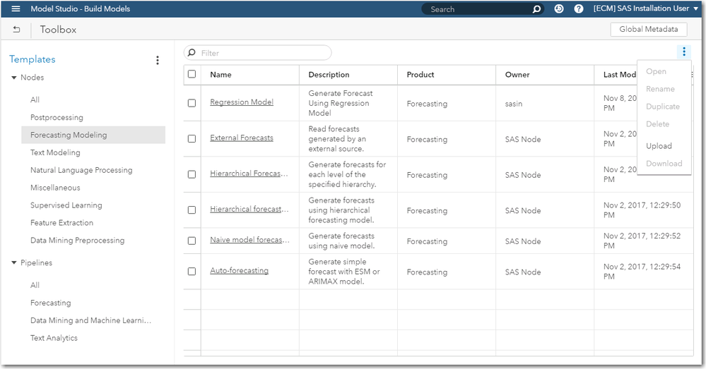
Once you add the three files of the pluggable modeling strategy in a Zip file, you can upload it to the Toolbox to use in the pipeline.

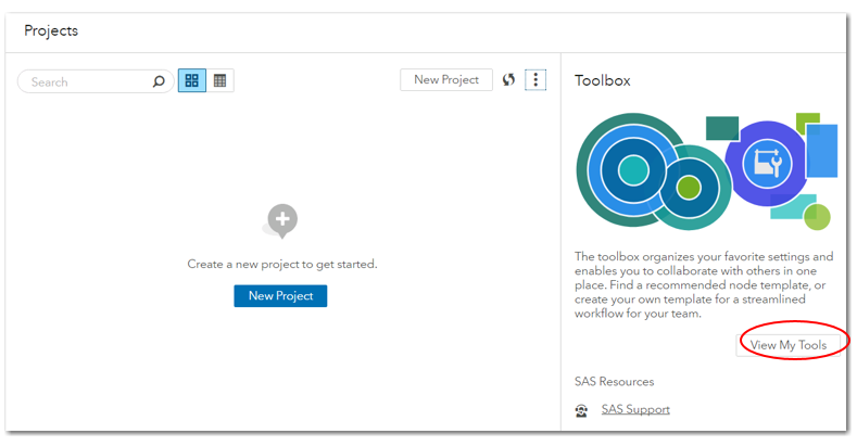
On the Model Studio interface, click on “View My Tools” button displayed in Toolbox session, see below.

In the toolbox interface, click on the three dots in upper right corner of the page to bring up toolbox menu. Select “upload” option, it will pop out a browse window. Select the zip file of the pluggable model you wish to upload, click OK.

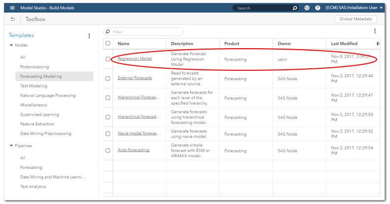
Once the pluggable modeling strategy is successfully uploaded, it will show up under the Forecasting Modeling Node:

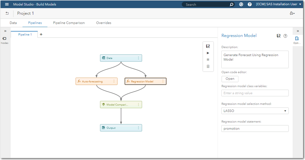
The pluggable model (Regression Model in this example) becomes available when you build a VF pipeline:

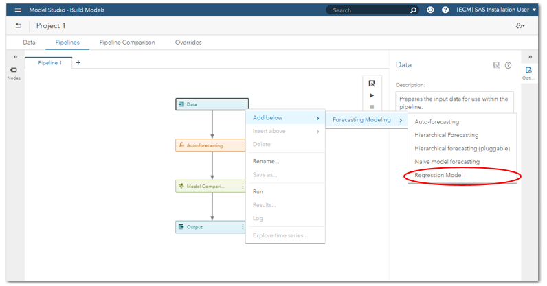
You can add a modeling node using the pluggable model. When the modeling node is selected, related info is displayed in the size panel, where you can view code or change the spec settings in the side panel. In the following screen, all three spec settings defined in regression model are correctly displayed, and are ready to take input from users.

Checklist

Here’s a quick checklist to sort out everything required to build a pluggable modeling node:

A zip file which contains three files: template.json, validation.xml, code.sas
Make sure the code takes input tables and generates output tables following the I/O contracts
Upload the zip file to Toolbox
The pluggable model is ready to use in the pipeline