- Home
- /
- SAS Communities Library
- /
- Using network projection to infer new links
- RSS Feed
- Mark as New
- Mark as Read
- Bookmark
- Subscribe
- Printer Friendly Page
- Report Inappropriate Content
Using network projection to infer new links
- Article History
- RSS Feed
- Mark as New
- Mark as Read
- Bookmark
- Subscribe
- Printer Friendly Page
- Report Inappropriate Content
What is Network Projection?
In network science, projections are used to infer linkages based on connection to a mutual entity. In the real world, network projections can be used to make personalized product recommendations or identify drug candidates that have the potential to reach a clinical trial.
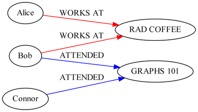
To give a social network example, consider Alice, Bob and Connor. Perhaps Alice and Bob work at the same coffee shop, and Bob and Connor have attended the same university course. These facts could result in inferred links between Alice and Bob or between Bob and Connor, respectively.

By applying projection over an employee-employer network (red links), you could infer the coworker link relationship, or by applying projection over a student-course enrollment network (blue links), you could infer the classmate link relationship.
A network like the first one, where entities on one side (or partition) link only to entities on the other side (or partition) is called a bipartite network. The result of a network projection is a one-partition (or unipartite) network of inferred links. And in SAS Viya, the Network Action Set has a handy action called projection to infer links based on input networks with bipartite relationships.
How to use the projection action
The following examples are intended to get you started with the PROC NETWORK projection statement syntax. Note that PROC NETWORK calls the projection action internally, so whether you use the PROC NETWORK syntax or the projection action syntax, the same algorithm runs. For more detail, you can view the network projection details documentation, and for end-to-end working example code, please follow along at GitHub.
Example: Network projection of an undirected bipartite graph
See the full example on GitHub [python][sas].
This section illustrates the use of the network projection algorithm on the bipartite graph G, which has two partitions {A,B,C,D,E} and {1,2,3,4,5,6}.

In order to use the Network Action Set, you must represent this graph as a table of links.
Table 1: mycas.Links
| from | to |
| A | 1 |
| A | 2 |
| A | 3 |
| B | 1 |
| B | 2 |
| B | 4 |
| B | 5 |
| C | 2 |
| C | 3 |
| C | 4 |
| C | 5 |
| D | 3 |
| D | 5 |
| E | 4 |
| E | 5 |
| E | 6 |
In order to perform a projection, we need to first tell the projection which of the two partitions to keep. To accomplish this, specify a table of nodes with a special column indicating the partition flag. The nodes flagged with the value 1 will be kept in the projected output while the nodes flagged with the value 0 will be considered as common neighbors for the sake of inferring links.
Table 2: mycas.Nodes
| node | partitionFlag |
| A | 1 |
| B | 1 |
| C | 1 |
| D | 1 |
| E | 1 |
| 1 | 0 |
| 2 | 0 |
| 3 | 0 |
| 4 | 0 |
| 5 | 0 |
| 6 | 0 |
You can use the syntax below to compute a projection based on the network provided via the nodes and links tables.
proc network
   links                 = mycas.Links
   nodes                 = mycas.Nodes;
   projection
      partition          = partitionFlag
      outProjectionLinks = mycas.ProjLinksOut
      outNeighborsList   = mycas.ProjNeighborsOut
      commonNeighbors    = true;
run;
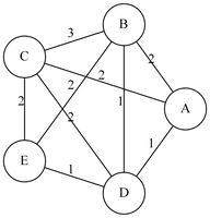
After the completion of those statements, the table mycas.ProjLinksOut is populated with the inferred links. For each link, because the option COMMONNEIGHBORS=TRUE is specified, the table also contains a weighting column that is equal to the count of shared neighbors among the {1,2,3,4,5,6} partition for each pair of nodes.
Table 3: mycas.ProjLinksOut
| from | to | commonNeighbors |
| A | B | 2 |
| A | C | 2 |
| A | D | 1 |
| B | C | 3 |
| B | D | 1 |
| B | E | 2 |
| C | D | 2 |
| C | E | 2 |
| D | E | 1 |
Projected graphs are often a simplification in that they carry less information than the bipartite input graph. The second output table, mycas.ProjNeighborsOut, preserves additional information by providing a list of the particular neighbors in the {1,2,3,4,5,6} partition that each node pair has in common.
Table 4: mycas.ProjNeighborsOut
| from | to | neighbor_id | neighbor |
| A | B | 1 | 1 |
| A | B | 2 | 2 |
| A | C | 1 | 2 |
| A | C | 2 | 3 |
| A | D | 1 | 3 |
| B | C | 1 | 2 |
| B | C | 2 | 4 |
| B | C | 3 | 5 |
| B | D | 1 | 5 |
| B | E | 1 | 4 |
| B | E | 2 | 5 |
| C | D | 1 | 3 |
| C | D | 2 | 5 |
| C | E | 1 | 4 |
| C | E | 2 | 5 |
| D | E | 1 | 5 |
The output, a unipartite weighted network, is visualized below:
Scale to bigger data
See the full example on GitHub [python][sas]
One of the strengths of SAS Viya is the ability to scale to large data sets. To illustrate the projection algorithm at large scale, consider the Amazon Movies and TV reviews data set, which you can download from here. In this bipartite data set, links are between user nodes and product nodes, and the existence of a link from X to Y indicates that user X reviewed product Y. The task performed here is projection onto the product nodes, that is, linking pairs of products together that were reviewed by one or more common users.
This bipartite input network is of challenging size for the projection task. There are 4.0 million nodes and 8.8 million links in the input, and the number of operations required to compute the projection is 
With eight threads on one machine, the projection algorithm takes just under seven seconds to complete.
NOTE: The number of nodes in the input graph is 4008117.
NOTE: The number of links in the input graph is 8765568.
NOTE: Processing network projection using 8 threads across 1 machines.
NOTE: Processing projection used 6.72 (cpu: 24.52) seconds.
With a cluster of five machines, the same projection calculation takes less than two seconds.
NOTE: The number of nodes in the input graph is 4008117.
NOTE: The number of links in the input graph is 8765568.
NOTE: Processing network projection using 40 threads across 5 machines.
NOTE: Processing projection used 1.43 (cpu: 37.95) seconds.
With multiple threads and multiple machines, you can divide and conquer your way to faster execution times on large data sets.
- Mark as Read
- Mark as New
- Bookmark
- Permalink
- Report Inappropriate Content
Hi Brandon,
Well done!
@Roel ;
You remember that ODE assignment from a couple of months ago.
The above is another way to solve it.
Koen
- Mark as Read
- Mark as New
- Bookmark
- Permalink
- Report Inappropriate Content
Thanks Koen "@sbxkoenk"!
Catch up on SAS Innovate 2026
Dive into keynotes, announcements and breakthroughs on demand.
Explore Now →SAS AI and Machine Learning Courses
The rapid growth of AI technologies is driving an AI skills gap and demand for AI talent. Ready to grow your AI literacy? SAS offers free ways to get started for beginners, business leaders, and analytics professionals of all skill levels. Your future self will thank you.


