Tip: Understanding the Basic, Intermediate, and Advanced Modeling Methods in SAS® Rapid Predictive Modeler

[#1]

Have you used SAS Rapid Predictive Modeler (RPM), and ever wondered what the difference between the Basic, Intermediate, and Advanced modeling methods is? In this tip we will look at each of these methods after importing the RPM projects into Enterprise Miner™. For information on how to interpret the SAS Rapid Predictive Modeler results, please see Miguel Maldonado’s article Tip: How to interpret your SAS Rapid Predictive Modeler results.

To find written documentation of the SAS Rapid Predictive Modeler, including information on the modeling methods, you can open RPM in either Enterprise Guide or the SAS Add-In for Microsoft Office. Once open, there is a button titled “Help” that when clicked will take you to the documentation for Rapid Predictive Modeler. Combining the written help with the screenshots below may help further improve your understanding.

For the examples in this Tip, we are using the Cars data set found in the SASHELP library. In the RPM menus we have set MSRP to be the dependent variable, and we have set Invoice to be rejected.

In addition the diagrams for each modeling method are attached to this tip so that you can use the RPM framework for your own data mining projects.

Basic Modeling Method:

Let’s look at a screenshot of the basic modeling flow after it has been imported into SAS Enterprise Miner. We have outlined a portion of this flow in a blue rectangle for comparison to the intermediate and advanced modeling methods.

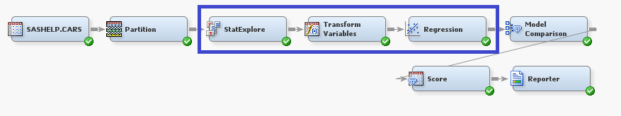
The first action in this flow is to partition the data into training and validation sets, at a 60-40 ratio. The StatExplore Node allows you to examine variable distributions in your data, and it can generate various plots and compute summary statistics. In the basic modeling method, the options for report generation have been turned off, and the StatExplore Node is set to select 100 variables. In the SASHELP.CARS data set, we have fewer than 100 variables, but for larger data sets, the StatExplore Node will reduce the number of variables in the basic modeling method.

In the Transform Variables Node, the interval inputs are transformed with optimal binning, and class inputs are transformed by grouping rare levels. The regression is a forwards logistic regression with no polynomial or interaction terms.

The basic modeling method is a short and simple method, which computes a regression after transforming the variables.

Intermediate Modeling Method:

Let’s now look at a screenshot of the intermediate modeling flow after it has been imported into SAS Enterprise Miner. In this flow we see a portion outlined in a blue rectangle and another portion outlined in a red rectangle with curved corners.

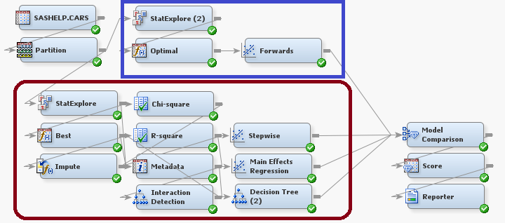
As you can see, this flow looks a lot busier than the basic modeling method. Notice that the node sequence outlined in the blue rectangle: StatExplore (2) -> Optimal -> Forwards is really just the basic modeling method! That is to say, the intermediate modeling method contains the basic modeling method and more. Let’s only consider the new nodes, those outlined in the curved corner rectangle, as we’ve already looked at the basic modeling method.

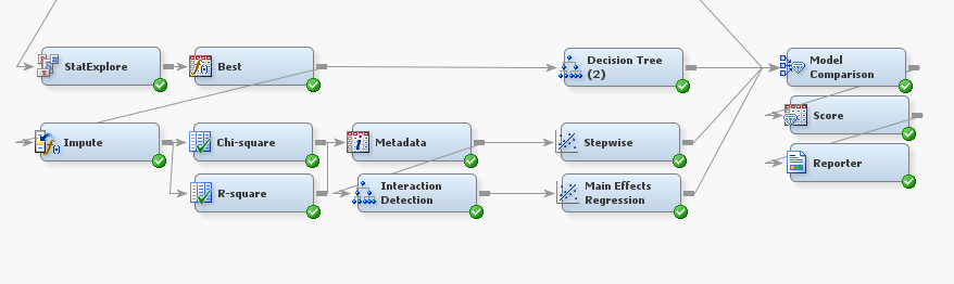
In the above picture we’ve zoomed in on the new portion of the intermediate modeling method. Like in the basic flow, we have a StatExplore Node. In this case, the StatExplore will select 200 variables as opposed to the 100 variables selected in the StatExplore Node for the basic modeling method. The Node labeled “Best” is a Transform Variables Node where the “Best” option (as defined by highest Chi Squared Test over several options) has been selected for transforming interval inputs.

After transforming the variables, we see that the flow splits into two paths. The first path is a decision tree to the model comparison node. The second path imputes missing values in the data, and then runs two variable selection methods, one based on chi-square and one on r-square. From the two Variable Selection Nodes we branch into a Regression Node that uses stepwise regression and a Tree Node. The Tree Node creates a new variable _NODE_, which is the leaf of the tree that an observation was placed into. This new variable and the rest of the data are used in the Regression Node titled “Main Effects Regression.”

The stepwise regression, the main effects regression, and the decision tree all lead to the Model Comparison Node, along with the resulting model from the basic modeling method. The Model Comparison Node will select the best model of the 4 input models to use as the Rapid Predictive Modeler model.

Advanced Modeling Method:

Finally we look at the advanced modeling method in SAS Enterprise Miner.

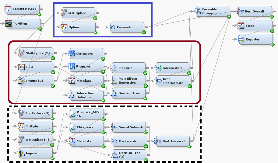
Again we see an increase in the complexity of the overall flow. There are three distinct portions of the flow. The node sequence outlined in the blue rectangle: StatExplore -> Optimal -> Forwards is from the basic modeling flow. The node sequence outlined in the red, curved corner, rectangle: StatExplore (2) -> Best -> … is from the intermediate modeling method. Thus, the advanced modeling flow contains everything from the intermediate modeling method and more. Let us zoom in on the new portions of the advanced modeling method, outlined in the dashed black rectangle.

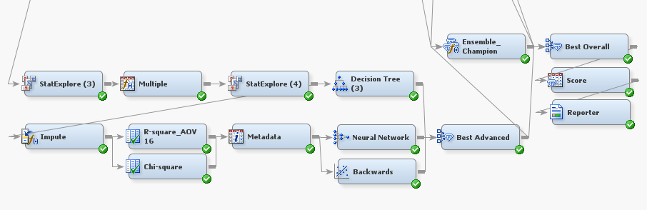
This portion of the method uses yet another StatExplore Node. In this portion of the flow, the StatExplore Node will select 500 variables, as compared to the 200 variables of the intermediate modeling method and the 100 variables of the basic modeling method. In addition, this StatExplore Node is set to generate reports on Interval variable distributions, Class variable distributions, and a level summary. These reports can be viewed in Enterprise Miner by right clicking on the node and clicking “Results.”

After the StatExplore Node is the Transform Variables Node, this time with the “Multiple” option for interval inputs. This means that the node creates multiple transforms for use with later modeling nodes. As in our discussion of the intermediate modeling method, we see a split in the flow. In one path we see a decision tree leading into a Model Comparison Node titled “Best Advanced.” In the other path we see the Impute Node, which will impute all the missing values. This is followed by two variable selection nodes that help to select the best variables using Chi-sqaure and R-square variable selection. After the variable selection nodes, the advanced modeling method computes both a neural network and a backwards regression.

The three models created by the decision tree, neural network, and backwards regression are compared in “Best Advanced” which picks the best model of those from the advanced modeling method portion. Let’s look at the last few nodes of the advanced modeling method.

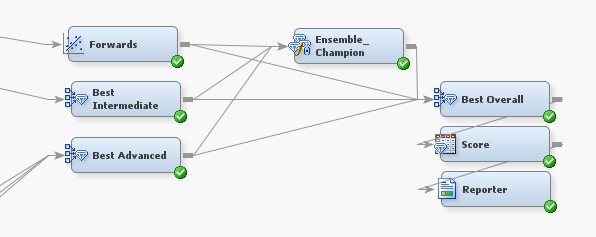
Here we first see the Regression Node titled “Forwards” and two Model Comparison Nodes titled “Best Intermediate” and “Best Advanced.” These are the results of the basic, intermediate and advanced portions of the overall flow. The best model of each partition is selected as a preliminary to picking a final model.

The Ensemble Node titled “Ensemble_Champion” creates an ensemble of the three input models by averaging the predicted values in the case of interval targets, or averaging probabilities in the case of class targets. Finally the Model Comparison Node “Best Overall” selects the best overall model from the four input models.

Concluding Remarks:

After looking at the basic, intermediate, and advanced modeling methods you may ask “Why wouldn’t I always use advance?” While it is true that the advanced modeling method will always be at least as good as the intermediate, which will in turn always be at least as good as the basic, the extra work takes extra time.

SAS Rapid Predictive Modeler seeks to give you a good balance between speed and model power! You can select a model based on your needs for how quickly you need an answer to your particular modeling problem. A quick review of the unique portions of each modeling method is presented below.

	Basic	Intermediate	Advanced
Variable Selection	StatExplore Node	StatExplore Node, Chi-square and R-Square criteria	StatExplore Node, Chi-square and R-square criteria
Variable Transformations	Optimal Binning	Optimal Binning, Best (as determined by Chi-square)	Optimal Binning, Best (as determined by Chi-square), and Multiple
Regression	Forwards	Forward, Stepwise, and Main Effects	Forward, Stepwise, Main Effects, and Backwards
Decision Tree	No	Yes	Yes
Neural Network	No	No	Yes
Ensemble of Models	No	No	Yes
Speed	Fastest		Slowest
Modeling Power	Least		Greatest

As a final note the Rapid Predictive Modeler will sample the data in the case of large data sets. This may include over-sampling in the case of rare event modeling.

Happy Modeling!

[Dmeatruis]

I am a new user to sas and i need help completeing some work

1.Clean the data set:

a.Eliminate all variables except GENHLTH, HLTHPLN1,

CHECKUP1,LASTDEN3, AGE, SEX, FLUSHOT5, and PNEUVAC3.

b.Create a two level variable based on FLUSHOT5 and PNEUVAC3 that

indicates any vaccination in the last year. Make 1 = Any vaccination and 2= No vaccination.

c.Delete observations from the data set that have a missing response to the

new vaccination variable.

d.Drop FLUSHOT5 and PNEUVAC3.

e.Make a label for the new vaccination variable.

f.Make formats for each of the variables left in the data set and apply them

in the data step.

2.Calculate the descriptive statistics for all variables in the data set you made in

question 1. Make sure the statistics have the appropriate title.

3.Create an appropriate graph to represent the distribution of responses for each

variable in the data set. Make sure the graphs have

anappropriate title