- Home
- /
- SAS Communities Library
- /
- The Usefulness of the Data Exploration Node in Model Studio
- RSS Feed
- Mark as New
- Mark as Read
- Bookmark
- Subscribe
- Printer Friendly Page
- Report Inappropriate Content
The Usefulness of the Data Exploration Node in Model Studio
- Article History
- RSS Feed
- Mark as New
- Mark as Read
- Bookmark
- Subscribe
- Printer Friendly Page
- Report Inappropriate Content
This article will show you how to use the Data Exploration Node in Model Studio. Similarly to PROC CONTENTS in Base SAS or the Multiplot node and the StatExplore node in Enterprise Miner, the Data Exploration node provides invaluable information about your data set and the distribution of the variables to help you create the best models and get the best results.
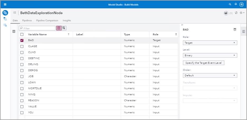
Let’s start by opening up Model Studio and setting up an Advanced template for the class target.
Mobile users: To view the images, select the "Full" version at the bottom of the page.
We will use the HMEQ data set and set BAD as a binary TARGET variable. The HMEQ data set is a home equity data set used to demonstrate SAS software. It has a variable BAD which is a 1,0 binary target indicating whether a person defaulted on their loan (1) or did not default (0). It also has a number of categorical and interval variables. Categorical variables include, for example, job and reason. Some of the interval variables are debt-to-income ratio (DEBTINC) and home value (VALUE).
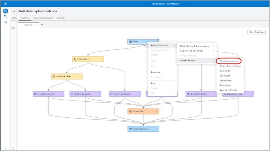
We can insert the Data Exploration node anywhere in our pipeline flow (except after the Model Comparison node). Let's start by putting a Data Exploration node immediately following the Data node. Right click the Data node, select Add child node, and select Miscellaneous to find the Data Exploration node.
Select the Data Exploration node and on the right side of your screen you can see you have a number of options. For example, under Input data partition you can choose if you want to look at all the data, test data, or training data. We’ll leave the default of All data.
Under Variable selection criterion you can choose either Importance or Screening. If you choose Importance, then you can choose the Maximum number of variables you want to explore.
Choose Screening as the Variable selection criterion to find anomalous variables--variables that don't fit the norm. You can choose screening cut offs to find variables with a lot of missing values, high cardinality, dominant levels, rare modes, or find variable distributions that are skewed or are abnormally tall and skinny, or short and fat. The Screening Results show tables of the anomalous variables and why they were determined to be anomalous.
For Interval Variables you can select the number of bins. For now we'll leave the default of eight. You can also select cluster plot and t-SNE projection. We'll leave those unchecked.
Right click and Run the Data Exploration node.
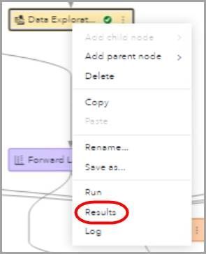
Right click again and select Results.
We arrive in the Summary tab. In the first box we see that we have no partitions and the number of observations is 5,960. In the next box we see the relative importance in a graph of each of our input variables. From this we can tell that the debt-to-income ratio is the most important variable by a large margin. Or so it seems at this point in our exploration!
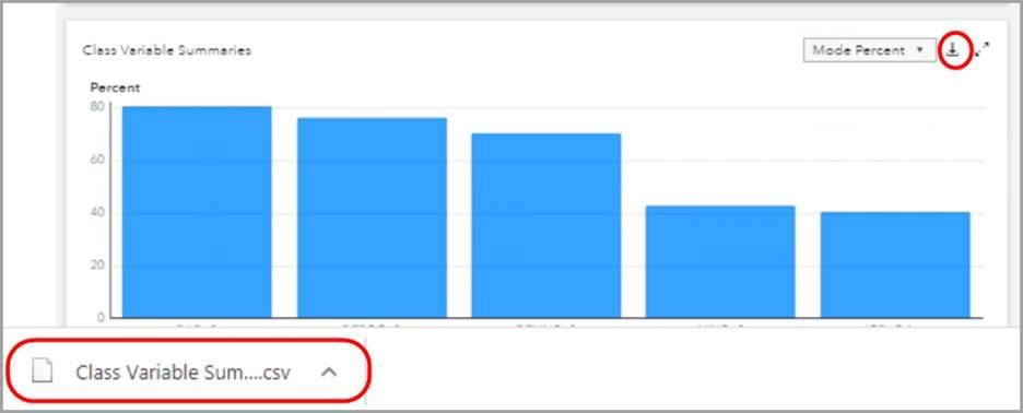
In our third box we have class variable summaries. We can look at either the cardinality or the mode percent.
Rolling over each bar shows the variable name, number of levels (cardinality), and hidden categories (yes or no).
Notice the download arrow that lets us download the data. Let's select mode percent and then select the download arrow. A CSV file is downloaded immediately.
Next we can see for each class variable what percentage of the observations fall into each level.
The next box shows us the interval variable moments. Because they're not really fitting in this small box let's expand using the two outward facing arrows to enlarge this box to full screen.
For each interval variable we can see the minimum, the maximum, the mean, the standard deviation, the skewness, the kurtosis, the relative variability, the mean plus 2 standard deviations and the mean minus 2 standard deviations in a nice neat table.
Next we can see the kurtosis plotted by the skewness for all of our interval variables. Notice how high the skewness is for home value (VALUE) and debt-to-income ratio (DEBTINC).
Recall that kurtosis means how narrow or wide the distribution is:
- Kurtosis > 0 indicates a tall, narrow distribution with few observations in the tails, i.e., leptokurtic
- Kurtosis = 0 indicates a normal distribution, i.e., mesokurtic
- Kurtosis < 0 indicates a flat distribution, heavy in the tails, i.e., platykurtic
Recall that skewness indicates if the distribution has a long left tail or a long right tail, as illustrated below.
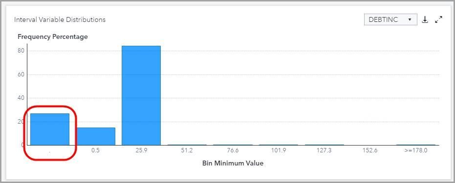
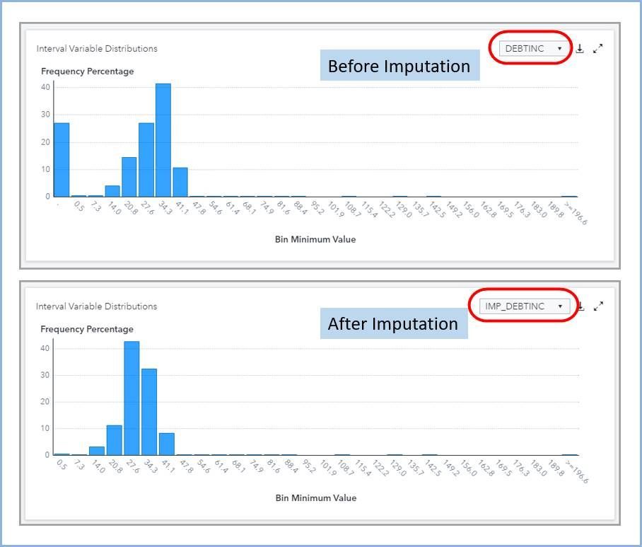
The next box is our interval variable distributions. This information on the interval variable distribution is quite useful because we can use our knowledge of statistics to see cases where we might want to impute or transform variables. For example if we look at debt-to-income ratio (DEBTINC), we see a large number of missing variables. In fact, more than 25% of the variables are missing or zero. This indicates that imputation might be helpful.
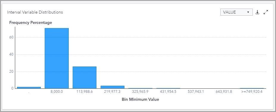
We will call from our interval variable summaries deviation from normality graph and our summary table that VALUE has a very high skewness; in fact it is a skewness over 3. Let's look at the graph of the distribution. We see below very distinctly this right skewness in the distribution of the VALUE variable. Based on our domain knowledge we are not surprised by this long right tail because very expensive homes are rarer than moderately priced homes.
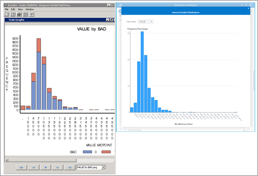
Let's go back and modify our data exploration node will select the node and in options on the right we will change under interval variables the number of bins to 18. Let's rerun the node and look at our results for Interval Variable Distributions for VALUE.
Quick quiz question for any legacy SAS users! What does this graph remind you of in EM?
Exactly! Enterprise Miner’s MultiPlot Node results.
Much of the same information that you have access to here from the Data Exploration Node in SAS Model Studio was available in Enterprise Miner from the MultiPlot node as well as the EM StatExplore node.
Our next graphic shows missing values in a bar chart. Wow! Look at how many missing values debt-to-income (DEBTINC) ratio has! Several other variables also have close to or over 10 percent missing values. This leads us to believe that our results might benefit from imputing missing values!
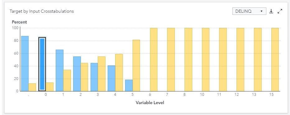
Next we see target by input cross tabulations . For example here looking at the delinquency variable DELINQ, We see a blue bar indicates no loan default (BAD = 0) whereas a yellow bar indicates the loan was defaulted (BAD =1) . On the vertical access we see the percent. We see that when the variable DELINQ is zero, most of our observations (> 80%) are not defaults (BAD = 0) and a small number (less than 20%) of our observations defaulted (BAD=1). In contrast, when DELINQ = 5, most of our observations (> 80%) are defaults (BAD = 1) and a small number (less than 20%) of our observations did not default (BAD=0).
Let's expand the properties table so that we can see the full table. Here Is some nice information including the VDMML version (dataMiningVersion) that we're using, Which in our case is version 2020.0.4. Some of the defaults are also shown such as a missing cutoff percent (missingCutoffPct) which is 25, the selection criterion which is IMPORTANCE, and so on.
Recall that PROC TREESPLIT is used to determine the variable importance. We can see information about the tree split procedure that has been used. For example, the split criterion is IGR, the Maximum branches per node is 2, etc. The IGR method uses the entropy metric to split each variable and then uses the information gain ratio (IGR) to determine the split.
We see that the debt-to-income ratio (DEBTINC) is by far and away the most important variable based on an initial look at the data.
But remember! We had a lot of missing values for debt-to-income ratio! So we might want to do some imputation.
You can display a three-dimensional nonlinear projection of interval inputs using t-Distributed Stochastic Neighbor Embedding (t-SNE). The t-SNE plot might help identify naturally occurring clusters in the data.
Replace this functionality of both the StatExplore node in enterprise miner and the Multiplot node in enterprise miner. So now you have two two two nodes in one!
Use Data Exploration Node To Evaluate Data After Imputation
Let's add a new data exploration node after the imputation node to see what changes we might see. Right click the imputation node add child node go to the miscellaneous group and pick the data exploration node. Right click and Rename this node Data Exploration After Imputation. On the right under options let's change the number of bins from the default of eight to 30 to be consistent with our previous data exploration node. Right click that new node to run it. After it runs right click again to see the results.
We are comforted to see that we still have 5960 observations. When we look at our relative importance we see that almost all of the variables have had imputed values added let's compare this relative importance graph to the one before imputation.
Notice that IMP_ is added before each variable that has had imputed variables Replace missing variables .
Quite a change! We see now that are variable for delinquent payments with imputed values added (IMP_DELINQ) Is now the most important instead of debt to income ratio. This is a great illustration of how important data preprocessing steps can be in your final results.
This article showed you just the tip of the iceberg of the usability of the data exploration node. But hopefully now your interest will be piqued and you'll explore more on your own and take advantage of this very handy node in Model Studio.
In a future post, I'll show how to use Model Studio's Transformation node, if the Data Exploration node indicates variables that might require transformation.
Catch up on SAS Innovate 2026
Dive into keynotes, announcements and breakthroughs on demand.
Explore Now →SAS AI and Machine Learning Courses
The rapid growth of AI technologies is driving an AI skills gap and demand for AI talent. Ready to grow your AI literacy? SAS offers free ways to get started for beginners, business leaders, and analytics professionals of all skill levels. Your future self will thank you.
- Find more articles tagged with:
- GEL


