- Home
- /
- SAS Communities Library
- /
- SAS Visual Scenario Designer 6.3 M1 Windows: The Aggregation Window
- RSS Feed
- Mark as New
- Mark as Read
- Bookmark
- Subscribe
- Printer Friendly Page
- Report Inappropriate Content
SAS Visual Scenario Designer 6.3 M1 Windows: The Aggregation Window
- Article History
- RSS Feed
- Mark as New
- Mark as Read
- Bookmark
- Subscribe
- Printer Friendly Page
- Report Inappropriate Content
The Aggregation Window
In the previous article, you were introduced to each type of window in SAS Visual Scenario Designer 6.3 M1, and you learned how the transformation window analyzes raw data to create detail data. This article introduces you to the aggregation window, and explains how it analyzes your raw data or detail data.
Here's a recap of the raw data that we're using for the examples in these articles:
Figure 1: Raw Data
|
Transaction ID |
Transaction Datetime |
Member ID |
Deposit Amount |
|
1 |
4/15/2014 8PM |
2 |
$5,000 |
|
2 |
5/1/2014 8AM |
2 |
$5,000 |
|
3 |
5/1/2014 12PM |
2 |
$4,000 |
|
4 |
5/1/2014 11PM |
3 |
$8,000 |
|
5 |
5/2/2014 1PM |
2 |
$5,000 |
|
6 |
5/3/2014 9AM |
1 |
$4,000 |
|
7 |
5/3/2014 5PM |
1 |
$2,000 |
|
8 |
5/3/2014 10PM |
3 |
$3,000 |
|
9 |
5/4/2014 11AM |
2 |
$4,000 |
|
10 |
5/4/2014 9PM |
3 |
$2,000 |
|
11 |
5/5/2014 11AM |
1 |
$3,000 |
|
12 |
5/6/2014 2PM |
1 |
$3,000 |
|
13 |
5/7/2014 10PM |
1 |
$2,500 |
|
14 |
5/8/2014 1PM |
2 |
$1,000 |
|
15 |
5/10/2014 10AM |
2 |
$2,000 |
|
16 |
5/10/2014 5PM |
2 |
$4,000 |
|
17 |
5/10/2014 8PM |
4 |
$12,000 |
|
18 |
5/12/2014 8AM |
2 |
$5,000 |
|
19 |
5/13/2014 4PM |
1 |
$2,000 |
Here again is the detail data that the transformation window outputs:
Figure 2: Detail Data from a Transformation Window
|
Transaction ID |
Transaction Datetime |
Member ID |
Deposit Amount |
|
1 |
4/15/2014 8PM |
2 |
$5,000 |
|
2 |
5/1/2014 8AM |
2 |
$5,000 |
|
3 |
5/1/2014 12PM |
2 |
$4,000 |
|
4 |
5/1/2014 11PM |
3 |
$8,000 |
|
5 |
5/2/2014 1PM |
2 |
$5,000 |
|
6 |
5/3/2014 9AM |
1 |
$4,000 |
|
9 |
5/4/2014 11AM |
2 |
$4,000 |
|
16 |
5/10/2014 5PM |
2 |
$4,000 |
|
17 |
5/10/2014 8PM |
4 |
$12,000 |
|
18 |
5/12/2014 8AM |
2 |
$5,000 |
How then does an aggregation window in SAS Visual Scenario Designer 6.3 M1 work? It summarizes raw or detail data across distinct category values, such as member ID, age or transaction type. The resulting data set includes one row for each unique combination of the category values.
An aggregation window uses group-by columns to aggregate, or segment, data into groups based upon the unique value in each group-by column. For example, selecting age and gender creates a grouping of age, and within age, a grouping of gender. Group-by columns are synonymous with partition keys, and are the level to which the data is aggregated. When you select one or more group-by columns, the resulting data set includes one row for each unique group-by column value. For example, if you applied a group-by column of day of the week, then you would have a data set of seven rows – one for each day of the week. The values that are associated with the group-by column or columns are automatically included in the resulting data set.
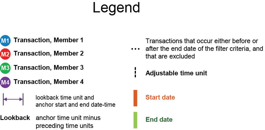
The legend below enables you to understand the elements in the animated image that follows.
Figure 3: Legend
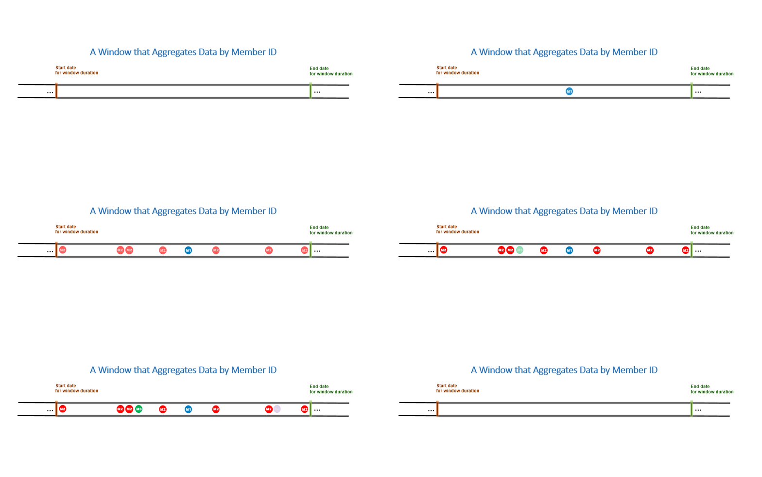
In the following image, a group-by column of Member ID has been applied to the detail data (as shown in Figure 2). As a result, Member ID is the group-by column that aggregates the data by Deposit Amount Sum and by Transaction Count.
Figure 4: Aggregating by Member ID
Figure 5 shows the aggregated Deposit Amount Sum and Transaction Count results from an aggregation window.
Figure 5: Aggregating Deposit Amount and Counting Transactions by Member ID
|
Member ID |
Deposit Amount Sum |
Transaction Count |
|
1 |
$4,000 |
1 |
|
2 |
$32,000 |
7 |
|
3 |
$8,000 |
1 |
|
4 |
$12,000 |
1 |
You might use an aggregation window to find total cash deposits per member that occur within the filter criteria.
This is article #2 in a five-part series. See the links below for the additional articles:
Part 1: Overview and Transformation Window
Part 3: Date-based Aggregation Window
Part 4: Transaction Window
SAS AI and Machine Learning Courses
The rapid growth of AI technologies is driving an AI skills gap and demand for AI talent. Ready to grow your AI literacy? SAS offers free ways to get started for beginners, business leaders, and analytics professionals of all skill levels. Your future self will thank you.
- Find more articles tagged with:
- data aggregation
- data visualization
- SAS LASR Analytic Server
- SAS Visual Analytics
- SAS Visual Scenario Designer


