Query Performance? Use a CAS Star Schema in SAS Viya 3.5

1 Like

Want to improve the performance of your query? Consider using a CAS star schema to join and perform on-demand calculations. Use a summary cas action to query and aggregate. Gains observed: reduce by almost 70% the time to join. Reduce data movement across CAS workers. Repeat the smaller dimensions at loading time and improve with 15% more your query performance.

The conclusions were derived on a star schema with one fact table and three dimensions, performing joins, on-demand calculations and aggregations.

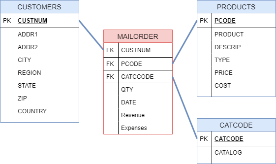
Star Schema Data Model

Select any image to see a larger version.
Mobile users: To view the images, select the "Full" version at the bottom of the page.

MAILORDER is the FACT table. PRODUCTS, CUSTOMERS and CATCODE are the dimensions.

A star schema is a join between one fact table and one or more dimension tables. Each dimension table is joined to the fact table through a key. Dimension tables are not joined to each other.

Data Volumes

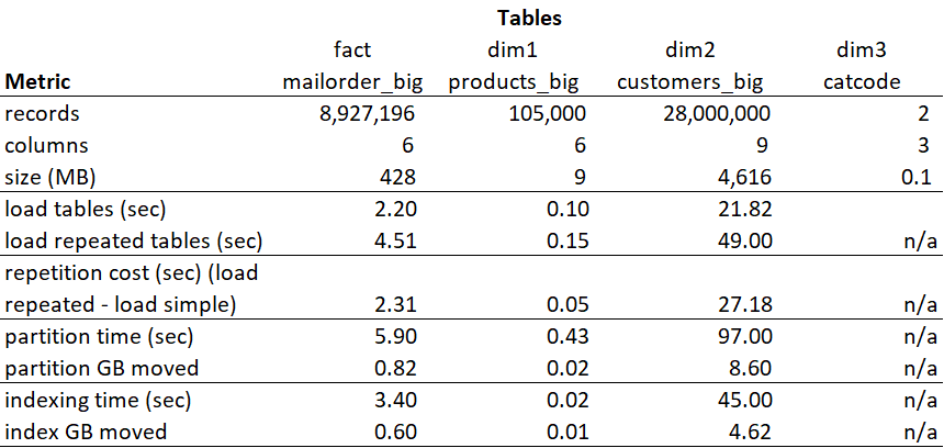
To test the star schema, I used the following tables: a decent fact table with 9 million records and a dimension with 28 million customers.

The time in seconds represents the real time displayed in the SAS log.

Metrics were gathered for loading, repetition, partitioning and indexing. Loading has to be performed in all cases. The last three are optimization techniques, but they come at a cost. The cost is measured in extra time and should be factored in.

In Automatic Data Loading with a CAS Data Source Star Schema in Viya 3.5, you will learn how to avoid loading before querying and create a star schema directly on data sources (files, database tables).

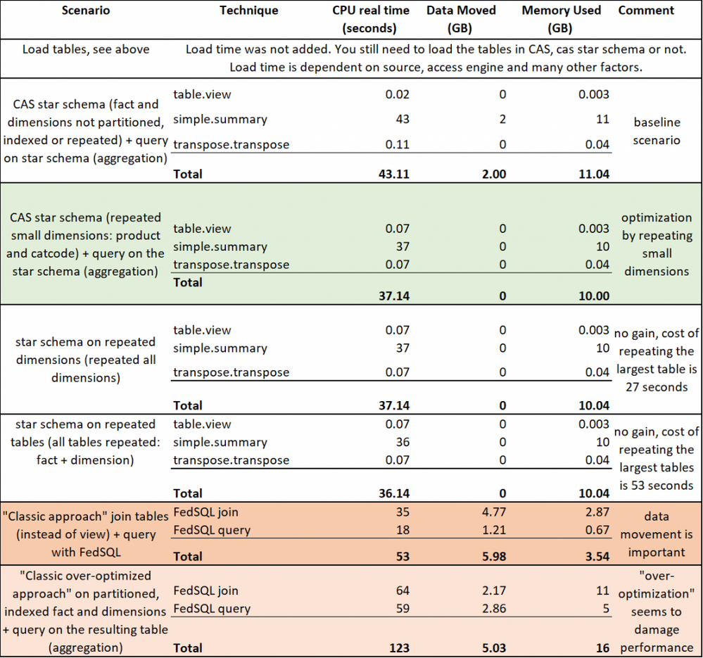
Scenarios Tested and Results

The leading scenario seems to be the second one, marked in green:

Repetition: the process to copy a small table, to be joined, on all workers. The join time is faster as data movement is reduced. Data is 'repeated' on all workers. More info in Stephen Foerster’s post.

Partition: the process to group rows on CAS worker nodes by commonly used BY-variables. More info in Stephen Foerster’s article and in Nicolas Robert’s article.

Indexation: the process to improve WHERE clause performance. More info in Stephen’s post.

Nicolas has found FedSQL the slowest in his aggregation tests on a big table. I found FedSQL comparable with a simple.summary followed by transpose.transpose cas action when many joins are needed.

CAS Star Schema: the leading scenario

Load the small dimensions as repeated tables

Tables are loaded, then replicated, copied on all workers (DUPLICATE=YES option in the data step). Again, this is OPTIONAL, but it seems to improve query performance. Credit goes to Uttam Kumar.

libname libcas cas caslib="casuser";
* Repeat with a Data Step;
options dscas dsaccel=any;
data libcas.CATCODE_REP (copies=0 replace=yes DUPLICATE=YES promote=yes);
set libcas.CATCODE;
run;

data libcas.PRODUCTS_BIG_NEW_REP (copies=0 replace=yes DUPLICATE=YES promote=yes);
set libcas.PRODUCTS_BIG_NEW;
run;

The rest of the tables are loaded normally. Copies=0 is used to reduce redundancy and hence, data movement. Repeated tables are used for join performance, not failover redundancy.

Create the CAS star schema

* Set OPTIONS;
options sessopts=(caslib="casuser" timeout=1800 locale="en_US" metrics="true");
* Leading scenario;
proc casutil;
droptable casdata="mail_view_opt" incaslib="casuser" quiet;
quit;
proc cas;
table.view / promote=true name='mail_view_opt'
tables={
{name='mailorder_big_new', varlist={'qty'}, as='m'},
{keys={'m_pcode = p_pcode'},
name='products_big_new_rep',  varlist={'price', 'cost', 'descrip', 'type'},
computedVars={{name="price_cost_ratio"}}, 
computedVarsProgram="price_cost_ratio = price/cost;", as='p'},
{keys={'m_custnum = c_custnum'},
name='customers_big_new',
varList={'addr1','addr2','city','country',
'region','state','zip'}, as='c'},
{keys={'m_catcode = cat_catcode'},
name='catcode_rep', varlist={'catalog'}, as='cat'}
};
quit;

Tables

The star schema is built as a view, MAIL_VIEW_OPT, on one fact and three dimensions. In this example, the CAS tables and the view are in the same CASLib ‘casuser’.

Aliases are defined for MAILORDER, PRODUCTS, CUSTOMERS, and CATCODE, namely "m", “p”, "c", and "cat", respectively. If you do not provide an alias for a component of a multi-table view, an alias is implied, namely "t1", "t2", and so forth.

Note the example uses the replicated tables PRODUCTS and CATCODE suffixed ‘_rep’.

Columns

Aliases (followed by underscores) are prepended to all variable names in the view, to help you identify which component table a column originated in. If you do not specify a list of variables for a component tables, all variables of that table are added to the view.

Computations

A computed column PRICE_COST_RATIO is defined for PRODUCTS. You can create computed columns by the same name for multiple component tables, the aliases are used to identify the columns uniquely. Notice that the computed columns evaluate independently for the component tables, you are not combining the scripts into one overall script for the view. If you wish to compute columns at the level of the view, then you can add computedVars and computedVarsProgram parameters to any action that uses the view.

Keys

The keys field is a list of strings of the form keyvar1 = keyvar2. You can specify multiple key variable pairs, but in a star schema, all keys need to resolve to the fact table. If there is ambiguity in the variable names, for example, if a variable appears multiple times across the tables, you use the alias as a prefix to identify the variable in a specific table. The key specification "pcode=m_pcode" means that the variable PCODE in the current table links to the variable PCODE in the component table aliased as "m". In this example, all key definitions map to the table aliased "m", this is the fact table of the star schema.

Query the Star Schema: use cas actions

Summary + transpose cas actions gave good performance, slightly better than FedSQL. Summary used by Visual Analytics for aggregations.

* Query with summary;
proc cas;
simple.summary result=r status=s/
groupByLimit=25000,inputs={{name="_va_d_v_Profit"},{name="m_QTY"},
{name="p_COST"},{name="p_PRICE"}},
orderBy={"p_TYPE","p_DESCRIP","c_STATE"},
orderByAgg={},orderByDesc={},subSet={"SUM"},
table={caslib="CASUSER",computedOnDemand="false",
computedVars={{name="_va_d_v_Profit"}},
computedVarsProgram="'_va_d_v_Profit'n=('m_QTY'n * ('p_PRICE'n - 'p_COST'n));;",
groupBy={{format="$.",name="p_TYPE"},{format="$.",name="p_DESCRIP"},
{format="$.",name="c_STATE"}},name="MAIL_VIEW_OPT"},
casout={name="mail_view_agg_va", caslib="casuser" replace=True};
if (s.severity == 0) then do; 
  transpose.transpose /
      table={name='mail_view_agg_va', caslib='casuser',
         groupBy={"p_TYPE","p_DESCRIP","c_STATE" }     },
      id={'_Column_'},
      casOut={name='MAIL_VIEW_BIG_TR', caslib='casuser', replace=true}, 
      transpose={'_Sum_'} ;
   end;
quit;
cas mySession terminate;

With a summary cas action you can calculate on-the-fly the profit, order and group by product type, product description and customer state. The result is the following:

CAS-Star-Schema-40-summary-cas-action-result--1024x150.png

Query the Star Schema: in a Visual Analytics report

A similar result can be achieved when you create a report in Visual Analytics:

CAS Star Schema Tips

Visual Analytics:

When dimensions or facts are updated, you need to recreate your star schema view (the operation is very fast)
If you have a Visual Analytics report on top of the star schema, you also need to refresh data in the report or, enable the 'Periodically reload page data' in the report page options
In Visual Analytics, if you use the star schema, all the tables, fact and dimensions must be promoted and accessible
If you alter the view and then use it in a report, Visual Analytics throws an error if you use altered view columns

Code:

The key between the fact and the dimensions must be one column (multiple join keys are not supported)
Drop the view before you recreate the star schema
Keys in the dimension tables must be unique. It sounds obvious, but in practice, you might have surprises, especially when you work with data you do not know. Check first, before you create the star schema.
In a scenario where the star schema content does not change often, but you have many users and frequent queries, and query performance is crucial, you can: 1/ create a star schema. 2/ partition the star schema, on the most frequent group variables. This is a cost, it takes on the above example 94-101 secs, lots of data is moved around, 27 GB, therefore, do it when feasible. The result is a table, not a view. 3/ Query the partitioned star schema (again, partitioning creates a table). The query is extremely fast: 0.18-0.19 sec with summary and transpose cas actions.

Conclusions

SAS Viya 3.5 and the CAS star schemas can help you gain time when you need to join multiple tables, aggregate or calculate on-demand. Advantages:

Star schemas + summary cas action: the fastest when you join and aggregate in your query. The cas actions table.view and simple.summary perform faster than Fed SQL or Data Step.
Data movement across workers is highly reduced.
Small dimensions duplicated on all workers seem to improve query performance.
You can further gain an improvement while duplicating all the tables, although the cost of repetition might not be really worth it.

Lastly, you need to understand what a CAS star schema is ‘sensible to’, to mitigate those factors.

Documentation and Useful Resources

Want to Learn More about Viya 3.5?

Acknowledgements: Stephen Foerster, Uttam Kumar, Nicolas Robert, and Mary Kathryn Queen for their contributions.

Thank you for your time reading this post. Please comment and share your experience with CAS Star Schemas and help others.

BJ · ‎03-04-2024

Hi Bogdan,

What would be the limitations to CAS star schema usage? Or what would be its sensitive points?

As this approach is very feasible to tackle a performance challenge, to what I should be aware of?

SASKiwi · ‎03-04-2024

CAS libraries store data in memory so you are limited by the amount of memory allocated to CAS. Also don't forget that you need to load your data into CAS memory from disk to start with. You want to avoid doing this every time you want to run your use case by maintaining the star schema in CAS with incremental updates.

Patrick · ‎03-04-2024

@Bogdan_Teleuca

The following statements are based on Viya 4 but I believe it's the same for Viya 3.5.

"Tables are loaded, then replicated, copied on all workers (DUPLICATE=YES option in the data step). Again, this is OPTIONAL, but it seems to improve query performance."

Afaik that's because all data blocks exists on all nodes and therefore no data movement between nodes is required.

"The rest of the tables are loaded normally. Copies=0 is used to reduce redundancy and hence, data movement."

I believe that's not true. Less copies means lower memory consumption but potentially more data movement with a cost to performance. Because the dimension tables are replicated such movement won't be necessary for the join in the view as such but depending on aggregations using the view less copies could lead to more data movement (like aggregation by a variable by which the underlying fact table is not partitioned).