- Home
- /
- SAS Communities Library
- /
- Imputing Missing Values is Easy in SAS Model Studio
- RSS Feed
- Mark as New
- Mark as Read
- Bookmark
- Subscribe
- Printer Friendly Page
- Report Inappropriate Content
Imputing Missing Values is Easy in SAS Model Studio
- Article History
- RSS Feed
- Mark as New
- Mark as Read
- Bookmark
- Subscribe
- Printer Friendly Page
- Report Inappropriate Content
A variety of imputation methods are available in SAS Model Studio for SAS Visual Data Mining and Machine Learning (VDMML). This blog will provide an overview of those built-in imputation methods.
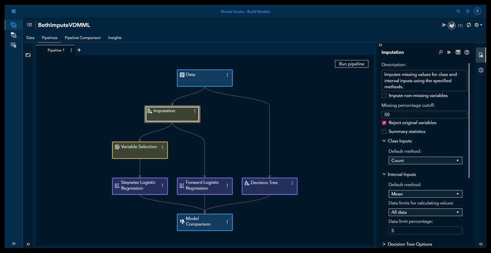
Let’s look at an example pipeline based on the software-provided template: Intermediate with Class Target. We are using the familiar HMEQ home equity data, with a binary target BAD. BAD = 1 meaning loan default, BAD = 0, meaning no default. Inputs include both class inputs like JOB and interval inputs like LOAN (loan amount).
Recall that some analytics methods are more sensitive to missing values than others are. Decision trees, for example, are robust to missing values. In contrast, neural networks and regressions are sensitive to missing values and can be highly affected. In fact, if you are missing even one value for one variable you can lose that whole row of data! Imputation can be essential in these situations.
SAS Model Studio let you choose from a whole host of imputation methods. See below a screenshot of our example pipeline. On the right you see we can impute both class inputs and interval inputs. The default method to impute class inputs is Count. The default method to impute interval inputs is the Mean.
Select any image to see a larger version.
Mobile users: To view the images, select the "Full" version at the bottom of the page.
Let's look a little more closely at the options we have. First, we have the option to Impute non-missing variables. By default this is not selected. Why would we we want to select this? This lets us generate an imputation score code regardless of the existence of missing values in the training data. We may like to select this because we anticipate that there are missing values in the validation or test data. We may need to impute those values to avoid losing observations.
The next option we see we have is to Reject original variables. We generally want to do this. This lets us replace the original variables with our new imputed variables. The next option is Summary statistics, which lets us see summary statistics in our results.
Class Inputs in the Imputation Node
We will use the imputation node to impute all our variables at once. The imputation node will impute everything EXCEPT those variables imputed individually in the Data tab (discussed at the end of the blog).
Now let's look at class inputs. We see the default is Count. Our other options as shown in the screen capture below are (none), Cluster count, Constant value, Decision tree, or Distribution.
If we select (none), then only the imputation methods that we specified specifically on the Data pane for individual variables would be performed.
If we select Cluster count the missing values will be replaced with that variable’s most frequent nonmissing value in the observations cluster. In order to use this method of imputation you must have a clustering node in the pipeline immediately preceding the imputation node. It is very easy to add that clustering node, as shown in the screen capture below.
Choosing Constant value means that you replace the missing values with a constant character. What would be a good example of that? Perhaps you have a situation where a region is always missing when the region is North for whatever reason. In that case you could simply replace your missing values for region with North.
Count is the default method. It means that the missing values are replaced with the input’s most frequent value.
Selecting Distribution means that you will replace the missing values with randomly selected values from an empirical distribution of the nonmissing values. So the first step is that SAS Model Studio creates a distribution of all of your values that are in the data set for that variable. Then SAS Model Studio randomly selects a value to replace each missing value. The benefit of this method is that you would not expect to significantly change the distribution of the data. The downside of this method is that if your data are if your training data are biased you could exacerbate that bias by using the training distribution to fill your missing values. This would be particularly harmful to your results if you have a lot of missing values and your training data are biased for this particular variable.
Interval Inputs in the Imputation Node
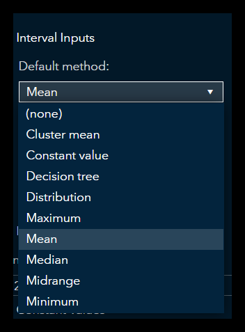
Now let's look at the interval inputs. As you see from the screen capture below, we have a few more options here.
Again we have the option of (none). Just as with the class inputs this option indicates that only imputations that you already specified on your Data pane are performed.
Next we have Cluster mean just as we did with our class inputs. This will indicate that the missing values will be replaced with the average of the observations cluster. Again you must have a clustering node in the pipeline immediately before the imputation node in order to select the Cluster mean.
Next we have Constant value. This means that you will replace the value with a constant number. You can select any constant number, or you can go with the default value which is zero. A great example of when this method is ideal is when you know that missing values are in fact supposed to be a certain number. For example, perhaps you know that in every situation in your data where there is a missing value for the number of late payments, you know that the actual value is zero. That would be a great example of when you could replace the class input with a missing number.
Next we have Distribution. This specifies that the missing value is replaced with a value that's randomly selected from an empirical distribution. This is an excellent method, but just as I mentioned previously, it can be dangerous if you have a lot of missing values and the non missing values are actually a biased subset of your full data set.
You can also select the maximum, the minimum, the mean, or the median. These are pretty self-explanatory. Another option is the midrange. The midrange is the maximum value plus the minimum value divided by two. This is not the same as the Mean! The Mean would be all of the nonmissing values added together and divided by the number of nonmissing values. The default method method is the mean.
You can also decide if you want to use all the data to calculate the imputed values, or if you want to get rid of your extreme values before calculating them (Data limits for calculating values). You can take care of your extreme values by either trimming or winsorizing your data set, as shown in the screen capture below.
The difference between winsorizing and trimming is that if you winsorize, you replace extreme values at the tails of a data set with the closest value next to them. Whereas in trimming you simply remove those values from the data set and do not replace them before calculating your mean, median, etc.
If you use winsorized or trimmed data, you must set a data limit percentage. This indicates what percentage of data are to be removed from both tails of the distribution. For example, if you set the data limit percentage to 5 (the default) that would create a 90% trimmed or winsorized data set. So the top 5% of data values and the bottom 5% of data values would be either simply cut from the data (trimmed) or replaced with the closest uncut value (winsorized). Assuming that your data are unbiased and representative of the population, winsorizing may be your preference.
Imputing Using Decision Trees
You can also use decision trees to impute variables. In this case you train a decision tree using all the other input variables in the data to predict the value of your input of interest. For example, to find the missing value for LOAN (loan amount), you would use all the other inputs to predict the loan amount. This predicted value is then the imputed value for LOAN.
A classification decision tree would use the chi square as the splitting criterion by default. A regression decision tree would use the F-test as the splitting criterion by default. For more information see the documentation and this post by Christian Medins.
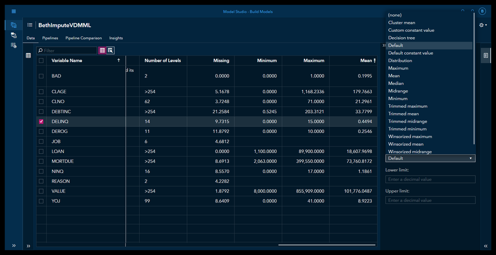
Using the Data tab to Impute Specific Variables
If you choose to impute specific variables in specific ways, you want to do this in the Data tab.
Summary
Imputing missing values can be very helpful, particularly when working with regressions, neural networks, and similar algorithms. SAS Model Studio for SAS Visual Data Mining and Machine Learning makes it easy to impute these values, using the methods of your choice.
For More Information
Notes:
Screen shots are from SSE Monthly Image Stable Version 2022.09. Release 20221025.1666685267102
Find more articles from SAS Global Enablement and Learning here.
Catch up on SAS Innovate 2026
Nearly 200 sessions are now available on demand with the SAS Innovate Digital Pass.
Explore Now →SAS AI and Machine Learning Courses
The rapid growth of AI technologies is driving an AI skills gap and demand for AI talent. Ready to grow your AI literacy? SAS offers free ways to get started for beginners, business leaders, and analytics professionals of all skill levels. Your future self will thank you.
- Find more articles tagged with:
- GEL


