- Home
- /
- SAS Communities Library
- /
- GLMs in SAS Dynamic Actuarial Modeling Solution
- RSS Feed
- Mark as New
- Mark as Read
- Bookmark
- Subscribe
- Printer Friendly Page
- Report Inappropriate Content
GLMs in SAS Dynamic Actuarial Modeling Solution
- Article History
- RSS Feed
- Mark as New
- Mark as Read
- Bookmark
- Subscribe
- Printer Friendly Page
- Report Inappropriate Content
Introduction
Insurance policies are designed to provide coverage for losses incurred by policyholders as a result of unforeseen circumstances. These occurrences, which occur sporadically over time, must occur while the policy is active to be considered eligible for coverage.
To establish a fair premium rate for a policy, actuaries need to quantify the stochastic elements inherent in the underlying claims process. This entails developing suitable probability models to assess both the frequency and magnitude of claims.
Random Variables, Probability Functions and Statistical Distributions
When dealing with a random phenomenon represented by a probability space, the focus often shifts towards specific numerical representations of outcomes within the sample space rather than the actual outcomes themselves. For instance, when viewing an insurance claim as the outcome of a random event, actuaries typically prioritize the financial value associated with the claim. Alternatively, they might emphasize the frequency of claims over the duration of the policy period.
The majority of random variables encountered in insurance modeling can generally be categorized into two main types – discrete (like claim frequency) or continuous (like claim severity). However, actuaries also encounter mixed variables, which incorporate elements of both discrete and continuous variables – for example, insurance payouts subjected to a deductible.
Given the nature of a random variable, we can also define mathematical functions that describes the likelihood of different outcomes of a random variable in a given random process. These functions are known as probability functions and they assign probabilities to each possible outcome of a random variables, indicating how likely they are to occur.
These probability functions are termed as probability distribution functions (pdf) in case of continuous random variables, and probability mass functions (pmf) in case of discrete random variables.
This brings us to the notion of a probability distribution or statistical distribution, which can be visualized as a comprehensive representation of the possible outcomes of a random variable along with their corresponding probabilities, derived from the previously outlined probability functions.
Significance of Probability Distributions or Statistical Distributions for Actuaries
Actuaries use probability distributions to model and analyze risks in a variety of contexts. For instance, in the insurance industry, actuaries use probability distributions to model the likelihood of different events, such as accidents or natural disasters, and to determine the appropriate premiums for insurance policies. In finance, actuaries use probability distributions to model the likelihood of different investment outcomes and to determine the appropriate levels of risk for different portfolios.
One of the key challenges of insurance modeling is to choose the most appropriate statistical or probability distribution to represent the frequency and severity of insurance claims. Different types of insurance claims may have different characteristics and patterns, such as the occurrence rate, the claim size distribution, and the presence of outliers or extreme values. Therefore, different statistical distributions may be more suitable for different types of insurance claims.
For insurance risk management, prudent choices about statistical distributions can help to measure and monitor the expected losses and the variability of losses for a given portfolio of policies. Appropriate assumptions about probability distributions can also help to control the risks by adjusting the policy terms, such as the deductible, the limit, and the coinsurance. These results can also help to determine the optimal reinsurance strategy, such as the type, the level, and the cost of reinsurance.
To achieve this, insurance companies rely on sophisticated modeling techniques that can handle the complexities and nuances of insurance data. One such powerful tool is the Generalized Linear Model (GLM).
Generalized Linear Models in Insurance Modeling
Suppose we want to develop pricing models for insurance products. We want to develop a model that can be used to predict quantifiable amounts of insurance risk. Most commonly used risk factors are claim frequency and claim severity.
Once we have determined the nature of the variable measuring risk and the factors that contribute to such risks, the next step involves establishing a structured framework to capture the relationship between the two.
For example, if we assume that there exists a linear relationship (in terms of parameters) between our measure of risk (let’s denote this as Y) and a set of contributing factors or predictors (collectively denoted as X) and if the measure of risk (Y) follows a statistically normal distribution, then we can estimate the relationship between risk and its contributing factors using a linear regression model:
Note: Linear regression is not commonly used for modeling insurance data. The reference here is primarily intended to conceptualize the modeling framework.
The primary objective of such a model would be to estimate the value of unknown parameters, β, from present and past data using a suitable estimation technique like Least Squares, Maximum Likelihood, etc. Once, the parameters (βs) are estimated we can then use them along with the chosen modeling framework to predict the values of Y.
The preliminary choice of models relies on prior understanding of the characteristics and structure of claims data. Furthermore, the commonly used measures of risk in such claim data do not conform to normal distributions. Typically, claim frequency is represented using non-negative discrete probability distributions, given that the count of claims is discrete and positive. On the other hand, it's commonly acknowledged that modeling claim severity is most effective when utilizing non-zero continuous distributions that exhibit right-skewness and heavy-tailed characteristics.
GLMs offer a more flexible approach compared to traditional linear regression models. They can accommodate non-normal distributions and handle different types of responses. This makes them particularly suitable for insurance modeling, where variables often exhibit skewed or categorical behavior.
GLMs deviate from linear regression modeling in three significant aspects:
- The distribution of the response variable is drawn from the exponential family. Consequently, the response distribution does not necessarily adhere to normality and can explicitly manifest non-normal characteristics.
- The relationship of interest between the transformed mean of the response and the explanatory variables is linear (in terms of the parameter).
- The variance of the response variable is a function of the response variables expected value. This allows for non-constant variance of the response variable (heteroskedastic) as opposed to homoscedastic assumption of linear regressions.
GLMs can be represented with the following equation:
Where g( ) is the link function that establishes the linear relation between the transformed mean of the response E[Y] and the explanatory variables (X). Furthermore, the link function g( ) must be differentiable and strictly monotonic such that the inverse g -1 ( ) exists, and
The above equation implies that the response variable E[Y] can be a nonlinear function of this linear combination explanatory variables (X) – that is, g( ) can be a non-linear function.
The distributions frequently employed by actuaries often exhibit a similar structure, allowing them to be classified into the exponential family. This characteristic has facilitated the development of a unified analytical framework known as Generalized Linear Models. For GLMs, response variable is assumed to have a probability distribution function from the exponential family that is given by:
θ is the parameter of interest (also termed as canonical parameter or natural parameter), Φ is the dispersion parameter. The functions b(θ), a() and C(Y, Φ) determine the type of distribution.
GLM Distribution Functions in SAS Dynamic Actuarial Modeling Ratemaking Node
Ratemaking involves the intricate task of establishing appropriate rates or premiums for individual insurance customers. Unlike conventional methods which may lack statistical sophistication, the Ratemaking node employs GLMs.
The Ratemaking node is specifically engineered for constructing GLMs tailored for insurance applications. It serves as a dedicated tool for actuarial pricing, offering a range of distributions from the exponential family suitable for various target variables. These variables often include frequency, severity, and pure premium, with the selection of distributions tailored to the nature of the target variables.
Claim Severity/Pure Premium Distributions
| Distribution | Range Requirements | Data Type |
|---|---|---|
| Burr | Nonnegative real values | Well-suited for modeling extreme values as a heavy-tailed distribution; effective for modeling insurance claim amounts that occur extremely infrequently. |
| Exponential | Nonnegative real values | Special case of the gamma distribution; appropriately suited for modeling thin-tailed distributions. |
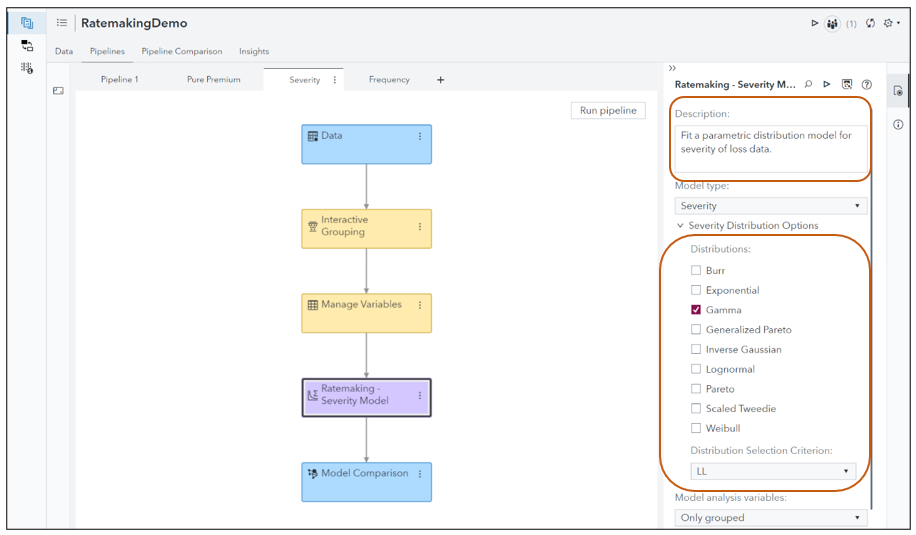
| Gamma | Nonnegative real values | Most suited for modeling insurance severity; default choice for severity modeling in the Ratemaking node. |
| Generalized Pareto | Positive real values | Suitable for modeling extreme claim severity amounts; focuses on upper tail value beyond a threshold value. |
| Inverse Gaussian | Nonnegative real values | A mixed discrete-continuous model, with a probability mass at zero and an Inverse Gaussian continuous component; suitable for modeling insurance claim sizes, including zero claims. |
| Lognormal | Positive real values | Suitable in situations (like fire, automobile collision) where the individual claim values can increase almost without limits but cannot fall below zero, with most of the values near the lower limit. |
| Pareto | Nonnegative real values | A special case of the Generalized Pareto Distribution (σ = Threshold). Suitable for modeling extreme claim severity values; default choice for modeling pure premium in the Ratemaking node. |
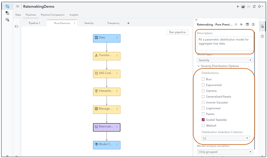
| Scaled Tweedie | Nonnegative real values | Suitable for modeling zero-inflated insurance claim data; uses a scale parameter to explain the influence of regressions on the scale parameter. |
| Weibull | Nonnegative real values | Suitable for left-truncated data; threshold value set by the deductible; if the claim values are less than the deductible, then it does not get recorded in the data. |
Select any image to see a larger version.
Mobile users: To view the images, select the "Full" version at the bottom of the page.
The ratemaking node for claim severity and pure premium modeling allows for multiple distribution specifications and various model selection criteria are available for selection of the champion model. The default distribution in case of claim severity modeling is the Gamma distribution and that in the case of pure premium modeling is Scaled Tweedie.
Claim Frequency Distributions
| Distribution | Range Requirements | Data Type |
|---|---|---|
| Poisson | Nonnegative integers | Suitable for modeling count of events occurring within a fixed time interval. |
| Conway-Maxwell-Poisson (CMP) | Nonnegative integers | Suitable for modeling count of events when claims frequency is often found to have a variance that is greater than the mean. |
| Negative Binomial (NB) | Positive integers | Suitable for modeling count of events when the mean is treated as a random variable. |
| Zero-inflated | Nonnegative integers | Suitable for Modeling zero-inflated count events; provides for a lower average premium for insurance customers with less risk as they are considered to have a high probability of making zero claims. |
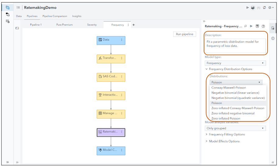
For claim frequency in the ratemaking node, we cannot specify multiple distributions (as in claim severity or pure premium modeling). The default distribution is Poisson.
Interpretability of GLM Models
The transparent structure and diagnostic capabilities of GLMs contribute to their interpretability. This makes it a valuable tool for communicating with the stakeholders.
- Parameter Interpretation: The coefficients in GLMs represent the relationship between the predictor variables and the response variable.
- Predictor Importance: GLMs allow for the assessment of predictor importance through the examination of coefficient magnitudes and significance levels.
- Model Diagnostics: GLMs offer various diagnostic tools such as residual analysis, leverage plots, and influence measures, which facilitate the evaluation of model fit and the identification of influential data points.
- Model Assumptions: GLMs come with well-defined assumptions, such as the linearity of predictors (in relation to the link function) and the independence of observations.
Challenges and Limitations of using GLMs
One hurdle lies in assuming a linear relationship between predictors and the response variable. However, this assumption may not hold true in all cases, necessitating either transformations of the data or the adoption of more adaptable modeling techniques.
Another issue is that of selecting the correct distribution family and link function. An erroneous pairing can result in biased estimates. Insurers must meticulously evaluate the attributes of the response variable and opt for the distribution family and link function that best align with its characteristics. This is somewhat mitigated in SAS DAM with the solution providing the option to compare various distributions and selecting the distribution (only for severity and pure premium models) that best fits the given data.
Furthermore, GLMs might encounter challenges related to overdispersion, wherein the variance of the response variable surpasses what is anticipated under the presumed distribution. Such circumstances can result in exaggerated standard errors and skewed estimates.
Conclusion
As the insurance landscape undergoes continual transformation, the utilization of GLMs in insurance modeling is likely to expand. Prospective avenues may entail integrating intricate interactions and non-linear associations, integrating external data sources for enhanced predictive efficacy, and crafting models that are adept at handling high-dimensional and unstructured data.
Additional Information
For more information on SAS Dynamic Actuarial Modeling visit the software information page here.
For more information on curated learnings paths on SAS Solutions and SAS Viya, visit the SAS Training page. You can also browse the catalog of SAS courses here.
Find more articles from SAS Global Enablement and Learning here.
Catch up on SAS Innovate 2026
Dive into keynotes, announcements and breakthroughs on demand.
Explore Now →SAS AI and Machine Learning Courses
The rapid growth of AI technologies is driving an AI skills gap and demand for AI talent. Ready to grow your AI literacy? SAS offers free ways to get started for beginners, business leaders, and analytics professionals of all skill levels. Your future self will thank you.
- Find more articles tagged with:
- Claim Frequency
- Claim Severity
- GEL
- generalized linear models
- glm
- Pure Premium
- Ratemaking
- SAS Dynamic Actuarial Modeling


