Determining CV among field sites in Proc Mixed

[#1]

How to determine which sites in a multi-site field campaign can be combined for analysis?

To answer this question, I return again to a data set that we tested for rate response and later unpacked the effect of combining trial sites.

Notably many of the standard textbook techniques fail to handle this simple and practical question of which sites can be combined, and which should be excluded.

Specifically, the assumption of normal distribution of residuals and equality of variance among groups was not grossly violated by examining various residual panels. And though each site shows a positive rate response of this treatment, by site differences interfered with sound interpretation. This was due, in fact, to inequality of variance.

How it works

In this blog we run proc mixed to fit our best model by location. We export covariance parameters, including the residual, which we use to calculate root mean squared error then percent coefficient of variation (%CV). We prefer site coefficients of variation over residuals because we don’t want to penalize sites with higher yield – we care more about relative variance among sites than absolute variance.

To do this, we use proc sql to conduct a table join between the covariance parameters table (covparms), and a table of means. Proc mixed furnishes the former table and proc means the latter table.

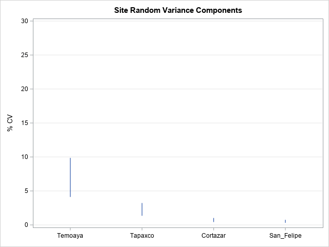
We go one step further to assist interpretation: covariance parameters (including the residual) are associated with 95% confidence intervals. We use that to calculate the upper and lower bound CV and display it on a highlow chart.

proc sort data=work.import;
by Location;
run;

proc mixed data=work.import CL=WALD;
	by 	Location;
	class Block Location;
	model Yield_tonnes_ha=Rate_kg_ha  /s covb outp=out ddfm=kr2; 
	random block / solution v;
	ods output covparms=covparms;
	/*IMPORTANT STEP: this exports the covariance parameters to a table. The covariance parameter table includes the residual*/
run;
quit;
/*Next we calculate the by-site mean - in this case of yield.*/
proc means
    data=import  mean noprint;
    by Location;
	Var Yield_tonnes_ha;
    output out=siteMeans (where=(_stat_='MEAN'));
run;
/*And then use proc sql to join the covparm2 table (including the residual to the mean*/
 proc sql;
    create table joined as 
    select a.*, b._stat_, b.Yield_tonnes_ha 
    from covparms a 
        left join siteMeans b
        on a.Location=b.Location
        where a.covParm='Residual';
quit;
/*And then use proc sql to join the covparm2 table (including the residual to the mean*/
data work.variance;
	set work.joined;
	/*The residuals are the mean squared error. We take the root mean squared error (rmse). We perform this calculation on the residual estimate, as well as its upper and lower bounds*/
	estrmse= sqrt(Estimate);
	lbrmse=  sqrt('Lower'n);
	ubrmse=  sqrt('Upper'n);
	/*And use that to derive the percent coefficient of variation = rmse/mean*100. Performing this calculation on the estimate, upper and lower bounds.*/
	estCV= (estrmse/Yield_tonnes_ha)*100;
	lowerCV= (lbrmse/Yield_tonnes_ha)*100;
	upperCV= (ubrmse/Yield_tonnes_ha)*100;
drop Subject Alpha _STAT_ estrmse lbrmse ubrmse Estimate 'Lower'n 'Upper'n;
run;
proc sort data=work.variance;
	by descending estCV Location;
run;
/*Let’s include the site %CVs as well as the site means following the proc mixed output*/
proc print data=work.variance;
title 'variance assessment';
run;
/*And display the by-site CV, represented as their 95% confidence intervals.*/
proc sgplot data=work.variance;
  highlow x=Location high=upperCV low=lowerCV;
  xaxis display=(nolabel);
  YAXIS LABEL = '% CV' GRID VALUES = (0 TO 30 BY 5); 
	TITLE "Site Random Variance Components"; 
  run;

Outcome

That’s it! Which sites would you combine? Certainly Cortazar and San Felipe which have very low variance and overlap nicely. Tapaxco has relatively variance too, though the 95% confidence interval does not overlap with the lower CV sites. Sometimes business requirements encourage combination of “more” sites, even at the expense of some precision of estimate. In any case, a combined analysis may justifiably exclude the CV outlier Temoaya.

Another facet to beware: sometimes site CV is represented as total variance over mean. This is not a fair comparison of sites in a mixed model context, because it would unduly penalize sites with a high treatment effect. What we care about is unexplained error after model fitting.

 

An additional aside, we sacrificed a degree of freedom at each site to block in an RCBD. Which sites most effectively blocked to isolate yield-affecting variance components?