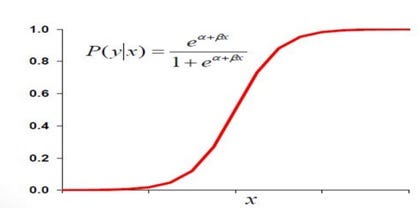
Logistic regression is a supervised machine learning classification algorithm that is used to predict the probability of a categorical dependent variable. The dependent variable is a binary variable that contains data coded as 1 (yes/true) or 0 (no/false), used as Binary classifier (not in regression). Logistic regression can make use of large numbers of features including continuous and discrete variables and non-linear features. In Logistic Regression, the Sigmoid (aka Logistic) Function is used.
We want a model that predicts probabilities between 0 and 1, that is, S-shaped. There are lots of S-shaped curves. We use the logistic model: Probability = 1 / [1 +exp (B0 + b1X)] or loge[P/(1-P)] = B0 +B1X. The function on left, loge[P/(1-P)], is called the logistic function.
Building a Logistic Model by using SAS Enterprise Guide
I am using Titanic dataset from Kaggle.com which contains a training and test dataset. Here, we will try to predict the classification — Survived or deceased. Our target variable is ‘survived’. I am using SAS Enterprise guide to analyze this dataset.
Setting the library path and importing the dataset using proc import
/* Setting the library path */
%let path=C:\dev\projects\SAS\PRACDATA;
libname PRAC “&path”;
/* Importing dataset using proc import */
proc import datafile = “C:/dev/projects/sas/pracdata/train.csv”
out = PRAC.titanic
dbms = CSV;
run;
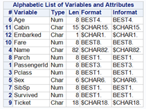
Checking the contents of the dataset by using proc contents function
/* Checking the contents of the data*/
proc contents data=work.train;
run;
We have 12 variables. Our target variable is ‘Survived’ which has 1 and 0. 1 for survived and 0 for not survived. Category variables: Cabin, sex, Pclass. Numeric Variables:Passenger ID, SibSp, Parch, Survived, Age and Fare. Text variable:Ticket and Name
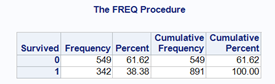
Checking the frequency of the target variable ‘Survived’ by using proc frequency
/* Checking the frequency of the Target Variable Survived */

proc freq data=work.train;

table Survived;

run;
We can clearly see that 342 people were survived and 549 people are not survived. A total number of observations = 891.
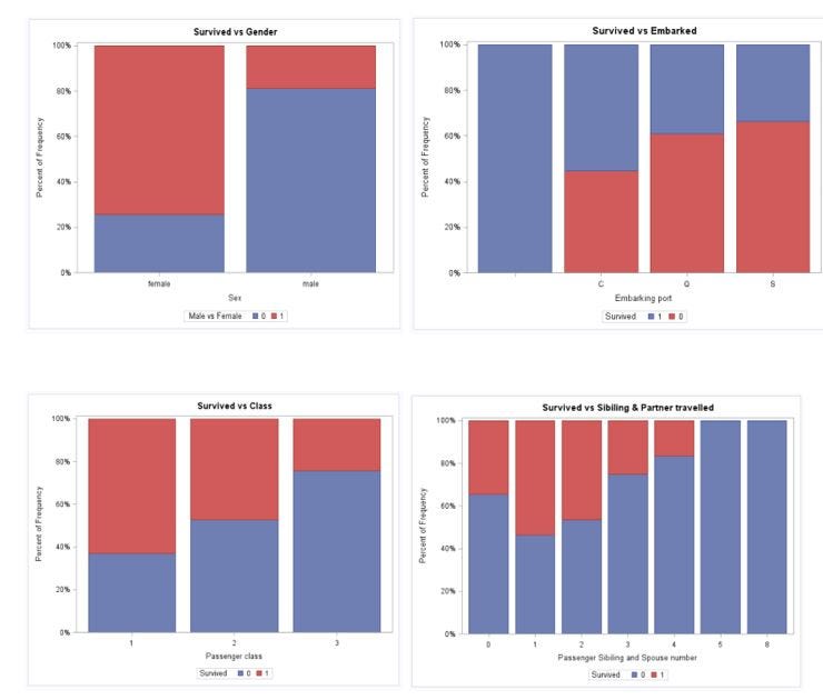
title "Survived vs Gender";
proc sgplot data=prac.titanic pctlevel=group;
vbar sex / group=Survived stat=percent missing;
label Embarked = "Passenger Embarking Port";
run;
Data Visualization
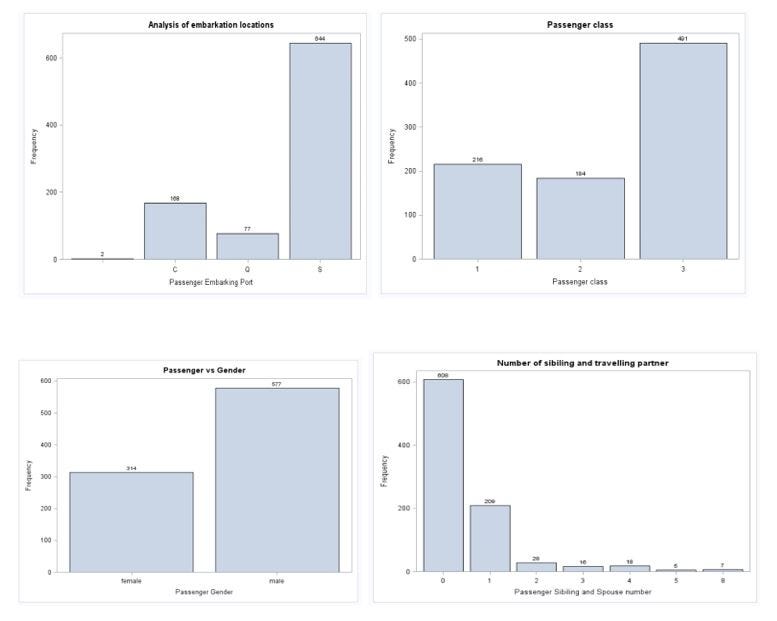
Normally, it is good practice to research with the data by using visualization. I am using proc sgplot to visualize the class, Embark.
title "Analysis of embarkation locations";
proc sgplot data=prac.titanic;
vbar Embarked / datalabel missing;
label Embarked = "Passenger Embarking Port";
run;
Nothing unusual can be seen in value distributions. Let’s analyze survived the rate with other variables.
title "Survived vs Gender";
proc sgplot data=prac.titanic pctlevel=group;
vbar sex / group=Survived stat=percent missing;
label Embarked = "Passenger Embarking Port";
run;
Here, we see a trend that more females survived than males. People travelled in class 3 died the most. Still, there are many ways to visualize the data. I am not going into detail.
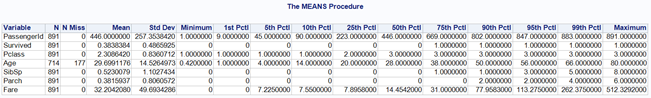
Checking the missing values by using proc means
/* Checking the missing value and Statistics of the dataset */
proc means data=work.train N Nmiss mean std min P1 P5 P10 P25 P50 P75 P90 P95 P99 max;
run;
We can see that Age has 177 missing values and no outliers detected.
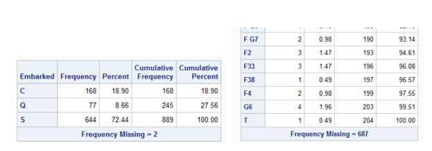
Checking for categorical variables:
title “Frequency tables for categorical variables in the training set”;
proc freq data=PRAC.TITANIC nlevels;
tables Survived; tables Sex; tables Pclass; tables SibSp; tables Parch; tables Embarked; tables Cabin;
run;
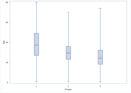
We have missing value in Age, Embarked and Cabin. We need to fill all missing age instead of dropping the missing rows. One way to filling by using mean age. However, we can check the average age by passenger class using a box plot. In SAS, we need to sort it out of the class and age variable before making it a box plot.
/* Sorting out the Pclass and Age for creating boxplot */
proc sort data=work.train out=sorted;
by Pclass descending Age;
run;
title ‘Box Plot for Age vs Class’;
proc boxplot data=sorted;
plot Age*Pclass;
run;
We can see the wealthier passengers in the higher classes tend to be older, which makes sense. We’ll use these average age values to impute based on Pclass for Age.
/* Imputing Mean value for the age column */
data work.train2;
set work.train;
if age=”.” and Pclass = 1 then age = 37;
else if age = “.” and Pclass = 2 then age = 29;
else if age = “.” and Pclass = 3 then age = 24;
run;
I have dropped the cabin variable as I don’t see it is going to impact our model and filled the missing value in ‘embarked’ using the median. (Selected median due to category variable).
Data Partition
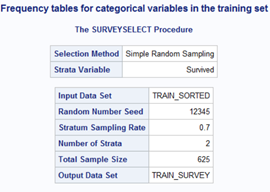
Splitting the dataset into training and validation by using the 70:30 ratio. First, I need to sort out the data usingproc sortand splitting by usingproc surveyselect.
/* Splitting the dataset into traning and validation using 70:30 ratio */
proc sort data = prac.train6 out = train_sorted;
by Survived;
run;
proc surveyselect data = train_sorted out = train_survey outall
samprate = 0.7 seed = 12345;
strata Survived;
run;
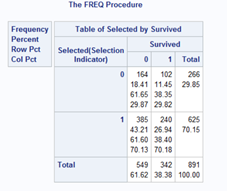
In order to verify the correct data partition, I am generating a frequency table by using proc freq.
/* Generating frequency table */
proc freq data = train_survey;
tables Selected*Survived;
run;
The Selected variable with the value of 1 will our target observation of the training part. Let us also perform quick set processing in order to leave only the columns that are interesting for us and name variables properly.
Building Model
We filled all our missing values and our dataset is ready for building a model. I am now creating a logistic regression model by usingproc logistic. Logistic regression is perfect for building a model for a binary variable. In our case, the target variable is survived.
/* Creating Logistic regression model */
proc logistic data=titanic descending;
where part=1;
class Embarked Parch Pclass Sex SibSp Survived;
model Survived(event=’1') = Age Fare Embarked Parch Pclass Sex SibSp /
selection=stepwise expb stb lackfit;
output out = temp p=new;
store titanic_logistic;
run;
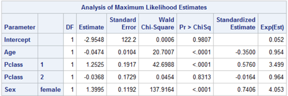
Good thing in SAS is that for categorical variables, we don’t need to create a dummy variable. Here we are able to declare all of our category variables in a class.
The variable selection algorithm decided that the model will include Age, Pclass and Sex variables.
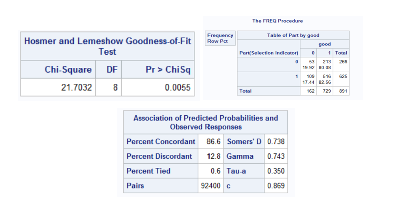
Good=1 is approximate both for the training set (Part=1) and validation set (Part=0). It amounts to 82.56% and 80.08% for the training and validation sets respectively. It is a stable model, however, if we see the Hosmer test the p-value is less. As per the book, higher, the p-value better the model fit.
If we can see the Concordant pairs, it is 86.6 %. Concordance is used to assess how well scorecards are separating the good and bad accounts in the development sample. The higher is the concordance, the larger is the separation of scores between good and bad accounts.
Testing test dataset
We can test our training model by using test dataset. It’s the same procedure for the importing test dataset in SAS by using Proc import and impute all the missing values.
Testing the test dataset by using our model
/* Testing with our model titanic_logisitic */
proc plm source=titanic_logistic;
score data=test1 out=test_scored predicted=p / ilink;
run;
Now we export the result into CSV file by using proc export. I separated the survived rate by using probability 0.5 and keeping only PassengerIdandSurvivedvariable in the result.
data test_scored;
set test_scored;
if p > 0.5 then Survived = 1;
else Survived = 0;
keep PassengerId Survived;
run;
/* Exporting the output into csv file */
proc export data=test_scored
file=”C:/dev/projects/sas/pracdata/Result.csv” replace;
run;
Only three variables were used in the model (age, class, and sex) and the result was 74.64 %. This is not a bad model; however, we have a large scope to improve the model by using other variables.
What’s next
In my next article, I will try to use other variables and improve the model. Also, we can apply other algorithms like decision tree, random forest to check the accuracy level. I will try to post in my next blog.
If you find any mistakes or improvement required, please feel free to comment.
Hi! Thank you for this nice guide! I'm trying to do the same but with my own data, but I don't really understand how to do the "where part=1;" under the section "building model". Is "part" a variable? And what does the 1 stand for?
Hi. I can't find the Kaggle dataset used for this tutorial. I can find literally 100's of Titanic datasets in Kaggle, but a lot of them have different variables and number of records. Is there a way to identify the actual dataset used in this example ?
The rapid growth of AI technologies is driving an AI skills gap and demand for AI talent. Ready to grow your AI literacy? SAS offers free ways to get started for beginners, business leaders, and analytics professionals of all skill levels. Your future self will thank you.