- Home
- /
- Programming
- /
- Graphics
- /
- Re: Overlay historgram and distributions
- RSS Feed
- Mark Topic as New
- Mark Topic as Read
- Float this Topic for Current User
- Bookmark
- Subscribe
- Mute
- Printer Friendly Page
- Mark as New
- Bookmark
- Subscribe
- Mute
- RSS Feed
- Permalink
- Report Inappropriate Content
I've read & studied some of Risk's posts about overlaying histograms/distributions, but still not getting it.
Been trying different things with Univariate, Capability, etc.
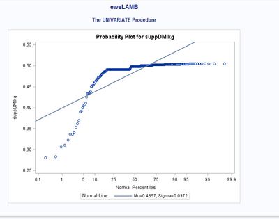
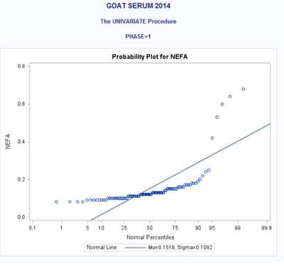
I have continuous data (supplement intake plot below) that I'm trying to fit various distributions (gamma, beta, lognormal, exponential, invgauss). Having trouble specifying mu = , sigma = , etc.
with help from the internet:
title 'supplement'; ods graphics on;
ods select histogram parameterestimates goodnessoffit fitquantiles;
proc univariate data = growth; var suppintake;
histogram / midpoints = 0.2 to 0.8 by 0.2
lognormal weibull gamm odstitle = title;
inset n mean (5.3) std = 'Std Dev' (5.3) skewness (5.3)
/pos = ne header = 'Summary Stats';
run;
I got the following to work, but none of the distributions fit the continuous data (feed intake)
DATA LAMB; SET grow;
PROC SORT; BY DAY ID JUN UREA;
RUN;QUIT;
ods graphics on;
ods select Histogram ParameterEstimates GoodnessOfFit FitQuantiles;
proc univariate;
var suppDMIkg;
histogram / midpoints=0.2 to 0.8 by 0.2
lognormal
weibull
gamma;
inset n mean(5.3) std='Std Dev'(5.3) skewness(5.3)
/ pos = ne header = 'Summary Statistics';
run;
Save
Accepted Solutions
- Mark as New
- Bookmark
- Subscribe
- Mute
- RSS Feed
- Permalink
- Report Inappropriate Content
There is nothing wrong with those notes in the log. They are not errors, just information. You can make the first NOTE go away by specifying lognormal(THETA=0).
As to the fit, by convention the distributions that we call lognormal, Weibull, and Gamma distributions have positive skewness.
However, your data have negative skewness, so the data distribution doesn't look anything like these theoretical distributions.
But that's no problem, because you can apply a linear transformation of the form x --> a - b*x. This will "flip" the direction of the tail of the data so that the data distribution can be modeled by the standard distributions.
For example, the following data step creates a new variable "OneMinusSuppDMIkg" that has the value 1-SuppDMIkg. This new variable has positive skew and the smallest value is 0.49 so you can model it as follows:
data A;
set growth;
OneMinusSuppDMIkg = 1 - suppDMIkg;
run;

proc univariate data=A;
histogram oneMinusSuppDMIkg / midpoints=0.475 to 0.8 by 0.025
          lognormal(theta=0.48)
          gamma(theta=0.48)
          weibull(theta=0.48);
run;
Equivalently, you could define Q = 0.52 - suppDMIkg and then use THETA=0 as the threashold.
Usually someone with domain knowledge can figure out a nice interpretable transformation. For example, if the measurements are "centimeters for a manufactured part," you might want to change units to "deviations less than the upper specification limit."
- Mark as New
- Bookmark
- Subscribe
- Mute
- RSS Feed
- Permalink
- Report Inappropriate Content
What is your question?
If you want to create a Q-Q plot, as in your images, then use the QQPLOT statement.
If you want to specify values for the parameter, rather than have the software find maximum likelihood estimates, then specify the parameter values in parentheses after the name of the distribution. For example:
HISTOGRAM / lognormal(mu=10 sigma=2) gamma(theta=0) weibull(theta=0 C=EST);
- Mark as New
- Bookmark
- Subscribe
- Mute
- RSS Feed
- Permalink
- Report Inappropriate Content
Hey Rick.
I initially posted & then edited (last part that I got to work).
I attached the data if needed.
My specific questions:
1. I guess that was my 1st question: how to specify mu sigma theta.
2. Any issues with the following log statements?
NOTE: Since a threshold parameter (THETA) was not specified for the lognormal fit for
suppDMIkg, a zero threshold is assumed.
NOTE: At least one W.D format was too small for the number to be printed. The decimal may
be shifted by the "BEST" format.
2. My data are continuous but for suppDMIkg (supplement intake), I can't get any distribution to fit & am thus, stuck.
Thanks for your time
- Mark as New
- Bookmark
- Subscribe
- Mute
- RSS Feed
- Permalink
- Report Inappropriate Content
There is nothing wrong with those notes in the log. They are not errors, just information. You can make the first NOTE go away by specifying lognormal(THETA=0).
As to the fit, by convention the distributions that we call lognormal, Weibull, and Gamma distributions have positive skewness.
However, your data have negative skewness, so the data distribution doesn't look anything like these theoretical distributions.
But that's no problem, because you can apply a linear transformation of the form x --> a - b*x. This will "flip" the direction of the tail of the data so that the data distribution can be modeled by the standard distributions.
For example, the following data step creates a new variable "OneMinusSuppDMIkg" that has the value 1-SuppDMIkg. This new variable has positive skew and the smallest value is 0.49 so you can model it as follows:
data A;
set growth;
OneMinusSuppDMIkg = 1 - suppDMIkg;
run;

proc univariate data=A;
histogram oneMinusSuppDMIkg / midpoints=0.475 to 0.8 by 0.025
          lognormal(theta=0.48)
          gamma(theta=0.48)
          weibull(theta=0.48);
run;
Equivalently, you could define Q = 0.52 - suppDMIkg and then use THETA=0 as the threashold.
Usually someone with domain knowledge can figure out a nice interpretable transformation. For example, if the measurements are "centimeters for a manufactured part," you might want to change units to "deviations less than the upper specification limit."
- Mark as New
- Bookmark
- Subscribe
- Mute
- RSS Feed
- Permalink
- Report Inappropriate Content
For additional thoughts, discussion, and an example of "reversing the distribution" when the data has negative skewness, see
"Sometimes you need to reverse the data before you fit a distribution."
Learn how use the CAT functions in SAS to join values from multiple variables into a single value.
Find more tutorials on the SAS Users YouTube channel.
SAS Training: Just a Click Away
Ready to level-up your skills? Choose your own adventure.


