In a previous Tip of the Week, my colleague Ray Wright showed how to use the %em_report macro to create custom graphs in a SAS Code node in SAS® Enterprise Miner™. Alternatively, you might have graphics from a SAS procedure or custom graphs you have created using ODS Graphics that you want to view and save to a file. The example below outlines how to display and save these graphics to a file (such as PDF or RTF) in a SAS Code node.
Here is the general form, for the code that can be used in an Enterprise Miner SAS Code node for embedding your graphic in an RTF or PDF file. You would just need to set the three macro variables at the top, and insert your code for creating ODS graphics where the comments indicate. I’ll go through two specific examples using this format.
%let name = /* name of the file to create (not including extension) */;
%let type= /* type of file: PDF or RTF */;
%let description = /* description for display in Results for SAS Code node */
%em_register(key=&name, type=FILE, extension=&type);
ods &type file="&&em_user_&name";
/* put code here that you use to generate ODS graphics */
/* end of code for ODS graphics */
ods &type close;
%em_report(key=&name, block=MODEL, viewtype=FILEVIEWER, autodisplay=Y, description=&description);
Example 1 – Using ODS graphics produced by a procedure
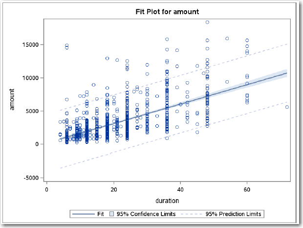
Many SAS procedures, including those in Base SAS and SAS/STAT, now produce graphs using ODS Graphics. As with ODS tables, some graphs are created by default, and some are created when certain procedure options are specified. This example uses the above code structure and shows how to view and save to a PDF file a graph created by the GLM procedure, The only differences are the values for the three macro variables at the beginning of the code and the code inserted to create the ODS graph.
The following code can be entered in the Training or Report Code pane of the SAS Code node Code Editor.
%let name = FitPlot;
%let type= PDF;
%let description = GLM Fit Plot;
%em_register(key=&name, type=FILE, extension=&type);
ods &type file="&&em_user_&name";
/* put code here that you use to generate ODS graphics */
/* For a single continuous predictor, PROC GLM creates a Fit Plot by default */
ods graphics on;
ods select FitPlot;
proc glm data=sampsio.dmagecr;
model amount = duration;
run;
quit;
ods graphics off;
ods select all;
/* end of code for ODS graphics */
ods &type close;
%em_report(key=&name, block=MODEL, viewtype=FILEVIEWER, autodisplay=Y, description=&description);
Click on the Run Node icon, then you will be able to open the Results window and click on the View button to open the PDF containing this Fit Plot from PROC GLM:
Example 2 – Using ODS Graphics procedures to create custom graphs
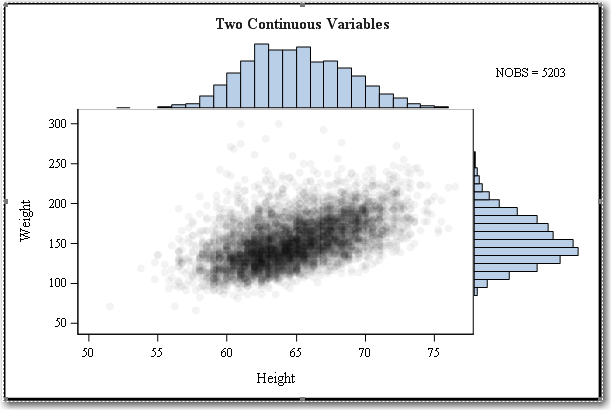
ODS Graphics provides a powerful way to create graphics as well. Many types of statistical graphs can be created using ODS Graphics procedures such as SGPLOT and SGSCATTER. Also, the Graph Template Language (GTL) can be used along with the SGRENDER procedure to create highly complex and custom graphs. The Graphics gallery available here displays some examples of these: http://support.sas.com/sassamples/graphgallery/index.html. Here is one of the examples, which produces a two-variable distribution plot, embedded into the code format given above to create an RTF file.
%let name = ScatterHist;
%let type= RTF;
%let description = Two-Variable Distribution Plot;
%em_register(key=&name, type=FILE, extension=&type);
ods &type file="&&em_user_&name";
/* put code here that you use to generate ODS graphics */
/* GTL code to define graph template */
proc template;
define statgraph scatterhist;
dynamic XVAR YVAR XTYPE YTYPE TITLE;
begingraph / designwidth=600px designheight=400px borderattrs=(thickness=3px);
entrytitle TITLE;
layout lattice / rows=2 columns=2 rowweights=(.2 .8) columnweights=(.8 .2)
rowdatarange=union columndatarange=union rowgutter=0 columngutter=0;
/* histogram or barchart at X2 axis position */
layout overlay / walldisplay=(fill) wallcolor=GraphBackground:color
xaxisopts=(display=none)
yaxisopts=(display=none offsetmin=0);
if (upcase(XTYPE) = "DISCRETE")
barchart x=XVAR / barwidth=1 stat=pct;
else
histogram XVAR / binaxis=false;
endif;
endlayout;
/* NOBS count cell */
layout overlay;
entry 'NOBS = ' eval(n(XVAR));
endlayout;
/* scatter plot with conditional axis types */
layout overlay / xaxisopts=(type=XTYPE) yaxisopts=(type=YTYPE);
scatterplot y=YVAR x=XVAR / datatransparency=.95
markerattrs=(symbol=circlefilled size=11px);
endlayout;
/* histogram or barchart at Y2 axis position */
layout overlay / walldisplay=(fill) wallcolor=GraphBackground:color
xaxisopts=(display=none offsetmin=0) yaxisopts=(display=none);
if (upcase(YTYPE) = "DISCRETE")
barchart x=YVAR / barwidth=1 orient=horizontal stat=pct;
else
histogram YVAR / orient=horizontal binaxis=false;
endif;
endlayout;
endlayout;
endgraph;
end;
run;
ods listing close;
proc sgrender data=sashelp.heart template=scatterhist;
dynamic YVAR="weight" XVAR="height" title="Two Continuous Variables";
run;
ods listing;
/* end of code for ODS graphics */
ods &type close;
%em_report(key=&name, block=MODEL, viewtype=FILEVIEWER, autodisplay=Y, description=&description);
You can again click the Run Node button and then view the Results when the run is complete. The graph that was created using GTL and PROC SGRENDER, shown below, is displayed and saved in an RTF file.