Data Science in Search for Best Predictions of Ski Tour Difficulties

[#1]

Use Case Description

Ski touring requires physical fitness, good equipment, technical skills and experience in assessing danger or difficulty in the terrain. Accidents are frequent. Some of them avoidable. www.skitourenguru.ch is a free of cost web service that publishes twice a day avalanche risk assessment and difficulty levels for backcountry ski tours in Switzerland. Its purpose is the reduction of avalanche and climbing accidents by means of adequate tour selection. The success of this service in Switzerland created demand in neighboring countries for Austria, Italy and France. An international extension is currently under construction. The Hackathlon use case focuses on the extension of tour difficulties to other countries.

The published technical tour difficulty level from the literature of the Swiss Alpine Club (SAC) is an important criterion for route selection. To extend this SAC metric to the entire Alpine region, the question arises if a machine learning method can determine tour difficulties consistent with the published SAC difficulties for the Swiss Alps and be applied to score tours in neighboring countries. Ideally such automatic method should provide full transparency about what determines the difficulty level of each ski tour (white box algorithm). Skitourenguru gathered the training data to explain the SAC difficulty levels of 1307 ski tours in Switzerland and scoring data from tours in neighboring countries. Each tour is decomposed into 10m segments, and their local topographic information such as slope, fall speed, forestation, curvature, etc. assigned from a digital elevation and landscape model.  Methods of machine learning, variable selection, linear optimization, in combination with statistical techniques might provide an answer to predict technical difficulty levels. The final model should extend the SAC difficulty metric to the entire Alpine area, but also localize and visualize the partial difficulties along each route on the map. 

Expected advantages are:

 1) consistent ratings without author or regional bias, 2) 

interpretability of difficulty ratings down to single segments of a tour, 3)

efficient initial- and reevaluation of large tour datasets                                                                                                         

*Click on the  Icon to embed your video*

Team Name	SiberianSnowTigers
Track	Data for Good
Use Case	Predictions of Ski Tour Difficulties
Technology	Data Science, Machine Learning, Statistics, Data Management
Region	EMEA
Team lead	Alice
Team members	Alice, Günter

[SnowTiger]

Code snippets from the Analysis of our Presentation:

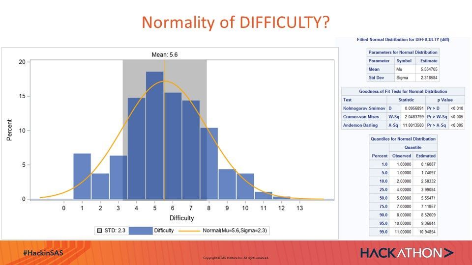
Visualization of Distribution of Dependent Variable DIFFICULTY:

ods graphics/height=400 width=700;
proc sgplot data=test3;
 title;* 'Distribution of Difficulty'; 
band y=difficulty lower=&std1. upper=&std2. /legendLabel="STD: 2.3" fillattrs=(color=silver); 
   needle x=DIFFICULTY y=percent/lineattrs=(thickness=38) transparency=.4 legendlabel="Difficulty";           ;
pbspline x=Difficulty y= Normal/nomarkers Lineattrs=(color=orange) Legendlabel="Normal(Mu=5.6,Sigma=2.3)";
*inset   "N=1307" "Mean=&mean_diff." "Median=&median_diff." "Std=&std_diff."/ OPAQUE;
   *label LoanType = 'Type of Loan';
   xaxis values=(0 to 13 by 1) Label="Difficulty";
   yaxis min=0;
   refline 5.554705/ axis=x Label="Mean: 5.6" Lineattrs=(color=orange);
   
run;

HPQUANTSELECT with Variable Selection based on AIC out of 94 Variables

proc hpquantselect data=mysasfil.Stg5_diff_ABT_ALL;
Title "Selection from 94 Predictor Candidates";
ods select fitstatistics parameterestimates ;
ods output Parameterestimates=PE;
class sac: Author_Grp_Bias;
model diff=Author_Grp_Bias SAC: ACCELM: ACCELS: CURVN: 
           CURVP: FOLDN: FOLDP: FOREST: FORESTSLOPE: RISK: 
           SLOPE: SPEEDM: SPEEDS: WIDTH: 
           x y z  count_am count_fm count_sm  
           StartEle StopEle Ele/ CLB Quantile=.5;
id id;
selection method=stepwise (CHOOSE=AIC);
partition Rolevar=TV(Train='0' Validate='1');
output out=QROut  P=P Residual=R COPYVARS=(_ALL_); 
run;

proc sql ;
select TV label="TV: 0=Trn 1=Val", 
count(R) as N, 
Mean(Abs(R)) AS MAE,
Mean(Round(abs(R),1)) as MARE,
sqrt(mean(R*R)) as RASE
from QRout group by TV; quit;

HPQUANTSELECT with Final Model:

proc hpquantselect data=mysasfil.Stg5_diff_ABT_ALL;
Title "Selection from Author_Bias, Risk_H Risk_M";
Title2 "Full Training N=1307, No Validation";
ods select fitstatistics parameterestimates ;
ods output Parameterestimates=PE;
class Author_Grp_Bias ;
model diff= Author_Grp_Bias RISK_M: RISK_H: / CLB Quantile=.5;
id id;
selection method=stepwise (CHOOSE=AIC);
output out=QROut  P=P Residual=R COPYVARS=(_ALL_); 
run;

Title "Prediction Error";
Footnote "Mean Absolute Error: MAE and Mean Abslute Rounded Error: MARE, Root Average Squared Error RASE";
proc sql ; select count(R) as N, Mean(Abs(R)) AS MAE,Mean(Round(abs(R),1)) as MARE, sqrt(mean(R*R)) as RASE 
from QRout ; quit;

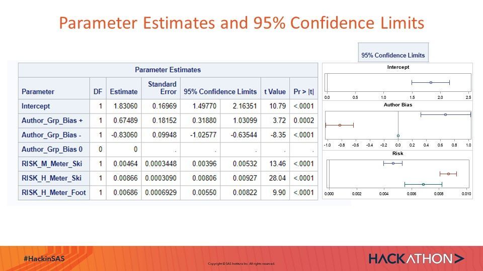
Visualization of Parameter Confidence Intervalls of Final Quantile Regression Model:

data pe;
set pe;
If scan(Effect,1,'_') eq 'RISK' Then Effect='Risk';
If scan(Effect,1,'_') eq 'Author' Then Effect='Author_Bias';
n=-_n_;
run;
ods graphics on/Height=100 width=300;
proc sgplot data=pe(where=(effect eq 'Risk')) ;
Title "Risk";
footnote;
 scatter y=n x=estimate / group=Parameter
 xerrorupper=UpperCl xerrorlower=lowerCL;
  refline  0 /axis=x;
 yaxis  display=(noticks nolabel novalues);
  xaxis display=(nolabel) values=(0 to 0.01 by 0.002);*Label="Estimates and 95% Confidence Interval" min=0;
* xaxis type=log offsetmin=0 offsetmax=0.3 min=0.01 max=100
 minor display=(nolabel);
  keylegend /Title="Parameter Estimates and 95% Confidence Intervals";
run;

ods graphics on/Height=100 width=300;
proc sgplot data=pe(where=(effect eq 'Intercept')) ;
Title "Intercept";
footnote;
 scatter y=n x=estimate / group=Parameter
 xerrorupper=UpperCl xerrorlower=lowerCL;
  refline  0 /axis=x;
 yaxis  display=(noticks nolabel novalues);
  xaxis display=(nolabel) values=(0 to 2.5 by .5);*Label="Estimates and 95% Confidence Interval" min=0;
* xaxis type=log offsetmin=0 offsetmax=0.3 min=0.01 max=100
 minor display=(nolabel);
  keylegend /Title="Parameter Estimates and 95% Confidence Intervals";
run;


ods graphics on/Height=100 width=300;
proc sgplot data=pe(where=(effect eq 'Author_Bias')) ;
Title "Author Bias";
footnote;
 scatter y=n x=estimate / group=Parameter
 xerrorupper=UpperCl xerrorlower=lowerCL;
  refline  0 /axis=x;
 yaxis  display=(noticks nolabel novalues);
  xaxis display=(nolabel) values=(-1 to 1 by .2);*Label="Estimates and 95% Confidence Interval" min=0;
  keylegend /Title="Parameter Estimates and 95% Confidence Intervals";
run;

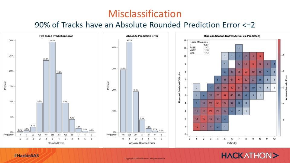
Visualization of Prediction Error and Prediction Misclassification:

ods graphics/height=700 width=600;
proc sgplot data=qrout noborder;
Title "Two Sided Prediction Error";
yaxis label= "Percent";
vbar ER/GROUPORDER=ascending stat=percent datalabel;
xaxistable ER / location=inside stat=freq ;
xaxis Label="Rounded Error";
run;

ods graphics/height=700 width=400;
proc sgplot data=qrout noborder;
Title "Absolute Prediction Error";
yaxis label= "Percent";
vbar ARE/GROUPORDER=ascending stat=percent datalabel;
xaxistable ARE / location=inside stat=freq ;
xaxis Label="Absolute Rounded Error";
run;

proc freq noprint data=qrout;
			Tables PR*Diff/out=score_freq_confusion outpct;
			run;
data score_freq_confusion;
set score_freq_confusion;
AbsoluteRoundedError=-abs(Round(diff-PR,1));
run;
ods graphics/height=700 width=700;
Proc sgplot data=score_freq_confusion;
Title "Misclassification Matrix (Actual vs. Predicted)";
inset ( "N"="1307" "RASE"="1.47" "MARE"="1.10" "MAE"="1.13")
   /Title="Error Measures" Valuealign=right LABELALIGN=left Border OPAQUE ;
heatmapparm y=PR x=diff colorresponse=AbsoluteRoundedError /outline   colormodel=(cxFAFBFE cx667FA2 cxD05B5B);;
   text x=diff y=PR  text=count / textattrs=(size=10pt) strip;
   gradlegend;
yaxis values=(0 to 12 by 1) Label="Rounded Predicted Difficulty";
xaxis values=(0 to 12 by 1) Label="Difficulty";
run;

[SnowTiger]

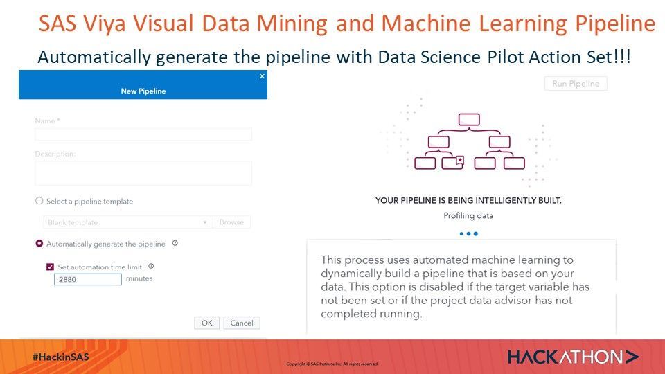
In search for most accurate prediction in this Use Case  we were successful with the automated machine learning pipeline exploration, execution and ranking in Viya  VDMML:

SAS Documentation of Data Science Pilot Action Set

Blog: https://blogs.sas.com/content/subconsciousmusings/2019/11/21/automated-machine-learning-pipelines/

Paper  SAS Global Forum SGF 2020, SAS4485-2020
Automation in SAS® Visual Data Mining and Machine Learning
Wendy Czika, Christian Medins, and Radhikha Myneni, SAS Institute Inc.

https://www.sas.com/content/dam/SAS/support/en/sas-global-forum-proceedings/2020/4485-2020.pdf

Video from SGF 2020

https://video.sas.com/detail/video/6145592076001/automation-in-sas-visual-data-mining-and-machine-le...

[SnowTiger]

Coverage of international extension of skitourenguru in the first German TV Channel  (outstation Bay...

Educational videos on how to use Skitourenguru

Press Room