- Home
- /
- SAS Communities Library
- /
- Using SAS Visual Analytics 8.5 to Explore Forecasting Data
- RSS Feed
- Mark as New
- Mark as Read
- Bookmark
- Subscribe
- Printer Friendly Page
- Report Inappropriate Content
Using SAS Visual Analytics 8.5 to Explore Forecasting Data
- Article History
- RSS Feed
- Mark as New
- Mark as Read
- Bookmark
- Subscribe
- Printer Friendly Page
- Report Inappropriate Content
Those of you who know me have heard me harp on the need to explore your data using SAS Visual Analytics as the very first step in your forecasting analysis.
Sometimes you find issues with the data that need to be addressed before you can use it for forecasting. Sometimes you find interesting relationships among variables that you want to include in your model, such as important underlying factors. This article demonstrates how I used SAS Visual Analytics 8.5 to explore some time series data that I got off the internet.
Data Source
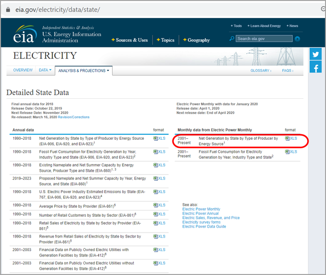
I pulled the data from the US Energy Information Administration web site as an Excel spreadsheet.
Select any image to see a larger version.
Mobile users: To view the images, select the "Full" version at the bottom of the page.
I did some rudimentary editing in the Excel spreadsheet (deleted rows above the header row, changed dashes to underscores in one of the sheet names) and then used SAS Studio to pull in all the sheets. I won’t describe that process here because I described it in my previous article Messy Data Prep: Old School Style in Viya 3.5. After going through the data exploration process, I will include my final data prep SAS Studio program for your convenience at the end of this post.
The data are monthly data for electricity generation in megawatt hours (mwh) by US state from 2001 to 2019 by energy source (coal, wind, etc.) by producer.
Explore Data Over Time
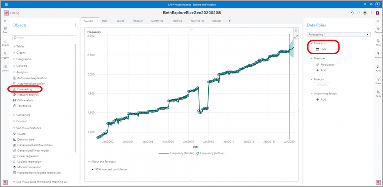
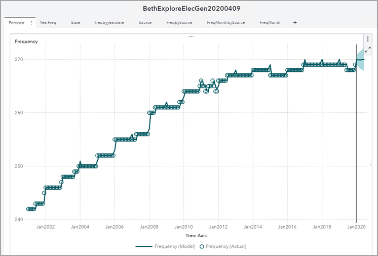
So let’s explore these data. We first use the forecasting object in Visual Analytics 8.5 to look at our data frequency over time by selecting date as my Time axis role. We see that the number of observations have increased steadily over time, which makes sense to me. More and more states are adding energy sources over time. But we see an anomalous drop in 2011 which might cause us pause and make us want to investigate further.
We also see that we get a close fitting ARIMA model. Note that SAS Visual Analytics provides preliminary forecasting results, but unlike SAS Visual Forecasting 8.5, we have no control over what model is selected. Recall that SAS Visual Analytics can be used as an exploratory tool for forecasting, but organizations that do many forecasts will want SAS Visual Forecasting also.
Month and Year should be Category not Measure variables, so let’s change them.
We can take a peak at our frequencies by year and then sort them by YEAR: Ascending.
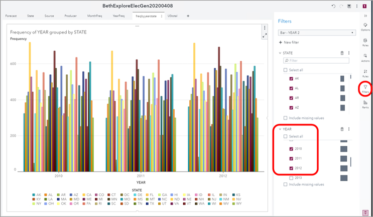
We can look at our frequencies by year and by state by adding State as my Group role. Here we also see that 2011 frequencies are lower for many states.
We can filter by year to zoom in on 2010, 2011 and 2012 only.
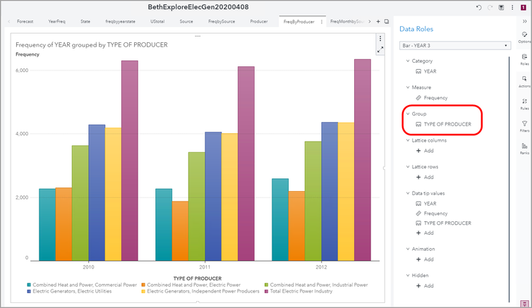
We can change our group to Type of Producer. Does your graph look the same as the one below? Did you remember to sort by YEAR: Ascending?
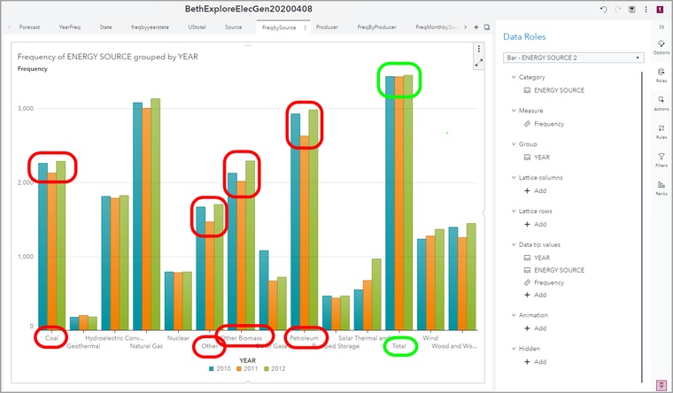
Let’s also take a look at the frequency of energy source grouped by year for 2010, 2011, and 2012. We see that although frequency of totals reported were similar over those three years. However, we can see that coal, other, other biomass, and petroleum had quite a bit fewer observations in 2011. Let’s shoot an email to EIA to find out if they know any reason for this frequency difference.
Notice something odd? We have two different groups for United States total: US-Total and US-TOTAL.
Let’s look at year grouped by state and filtered by just US-Total and US-TOTAL. We see easily from this graph that they changed from “US-TOTAL” to “US-Total” in 2012. But you can imagine how that might mess up our forecasting!
Note: We used the Options pane to change from horizontal to vertical bars.
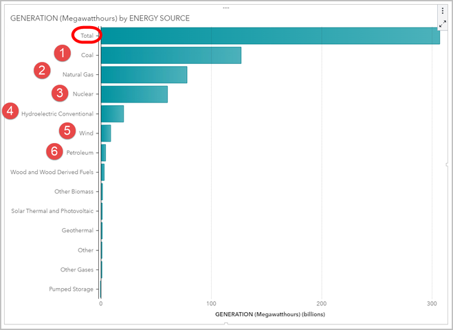
Let’s use Visual Analytics to see which sources are contributing to the largest electricity generation. We can than select the top ones to use in our analysis, leaving it uncluttered by the small timers. The top six are coal, natural gas, nuclear, hydroelectric, wind, and petroleum. I’ll filter the others out using my data prep program.
We see that there are a number of producer types, some of which subset each other. I am only interested in total electric power industry, so I will also filter the others out in my data preparation.
We can look at month frequencies by energy source, but it’s a bit busy.
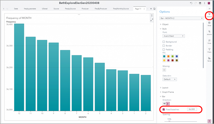
Let’s simplify and just look at frequency of month.
At the scale shown in the graph above, it looks very similar, so let’s set the y axis to start at 36,000.
Update data, and refresh
Now we have a much better understanding of the data, and some idiosyncrasies in it. I will finalize the data prep to ready the data for SAS Visual Forecasting. I won’t go into detail about that here, but see my article Messy Data Prep: Old School Style in Viya 3.5 . Also, for the uber-curious, I have included a copy of my SAS Studio program.
*************************************************************************************************
*																								*
*	IMPORT EXCEL SHEETS:  SAS Studio Sample Code															*
*	EIA Electricity Generation Monthly Data by US State 2001 to 2019 https://www.eia.gov/electricity/data/state/
*	Beth Ebersole																				*
*	05 APR 2020																					*
*																								*
*************************************************************************************************;
/*
proc setinit;
run;
options msglevel=I;
*/

* 1) Put EIA data on \\nagel01\gate\team\beeber\;
* 2) Upload folder in the SAS Studio Explorer tree...  intviya01 > Home > sasuser.viya > BethOut ;

libname bethout '/home/beeber/sasuser.viya/BethOut';

FILENAME REFFILE DISK '/home/beeber/sasuser.viya/ELECGEN2019.xlsx';
options symbolgen macrogen;
%macro elec(sheet);
proc sql;
%if %sysfunc(exist(WORK.elecgen&sheet)) %then %do;
    drop table WORK.elecgen&sheet;
%end;
%if %sysfunc(exist(WORK.elecgen&sheet,VIEW)) %then %do;
    drop view WORK.elecgen&sheet;
%end;
quit;
proc import datafile = reffile dbms=xlsx out=work.elecgen&sheet;
  sheet="&sheet";
  getnames = yes;
proc sort; by state year;
*proc print data=elecgen&sheet (obs=10); *title "&sheet";
%mend elec;
%elec(2001_2002_FINAL);
%elec(2003_2004_FINAL);
%elec(2005_2007_FINAL);
%elec(2008_2009_FINAL);
%elec(2010_2011_FINAL);
%elec(2012_Final);
%elec(2013_Final);
%elec(2014_Final);
%elec(2015_Final);
%elec(2016_Preliminary);
%elec(2017_Preliminary);
%elec(2018_Preliminary);
%elec(2019_Preliminary);
run;

data work.elecgen2019a (drop=day);
  set 	elecgen2001_2002_FINAL
		elecgen2003_2004_FINAL
		elecgen2005_2007_FINAL
		elecgen2008_2009_FINAL
		elecgen2010_2011_FINAL
		elecgen2012_Final
		elecgen2013_Final
		elecgen2014_Final
		elecgen2015_Final
		elecgen2016_Preliminary
		elecgen2017_Preliminary
		elecgen2018_Preliminary
		elecgen2019_Preliminary;
  *if state = " " then delete;
  day = 1;
  date = mdy(month,day,year);
  format date monyy.;
  yearsas=mdy(month, day, year);
  format yearsas year4.;
  rename 'ENERGY SOURCE'n=EnergySource
     	 'GENERATION (Megawatthours)'n=Generation_mwh
 		 'Type of Producer'n=ProducerType;

run;
data work.elecgen2019b;
  set elecgen2019a;
  if state ne "US-Total" and state ne "US-TOTAL";
  if substr(EnergySource,1,5) = "Hydro" then EnergySource = "Hydro";
run;


data work.elecgen2019c;
  set work.elecgen2019b;
  if ProducerType = "Total Electric Power Industry";
  if EnergySource = "Coal" or
     EnergySource = "Natural Gas" or
     EnergySource = "Nuclear" or
     EnergySource = "Hydro" or
     EnergySource = "Wind" or
     EnergySource = "Petroleum";
run;


data work.temp1;
  set work.elecgen2019c;
if 2010 <= year <= 2012;
if month = 12;
run;
proc contents data=work.temp1; run;
proc print data = work.temp1 (obs=5000); title 'temp1'; run;

data bethout.elecgen2019 (drop=ProducerType);
  set work.elecgen2019c;
run;

cas mysession sessopts=(caslib=casuser timeout=1800 locale="en_US");
proc casutil;
  droptable casdata="ELECGEN2019" quiet;
  load data=BethOut.elecgen2019 outcaslib = "casuser" casout="ELECGEN2019" promote;
  quit; *best practice is to close the CAS thread;
  run;
We can now Refresh the data source to our latest version.
And let’s take a peek at the frequency our new data over time.
We can also peek at a few of the individual forecasts by source and state. Everything looks hunky-dory.
At this point, we are comfortable enough with our data to put them into SAS Visual Forecasting 8.5. We’ll see that in my next article!
Summary
In summary, we have a plethora of objects in SAS Visual Analytics that are useful for exploring our time series data, including the Forecasting object. Exploring and getting to know our data is an essential first step to any time series analysis.
For More Information
Maybe you are sheltering in place during the Novel Coronavirus crisis with your boomeranged adult children, who are using up all the bandwidth in the house streaming a movie they “need to watch for college.” Or maybe your preschoolers’ day care is closed, and you hear “Daddy, Daddy, Daddy, pick me up” and “Mommy, Mommy, Mommy, look at this” from sunup til sundown. Or perhaps you have a needy spouse who thinks that because you are working from home, you should prepare gourmet meals and home-baked desserts nightly or they want you to fix that back porch step, because you “should have plenty of time now that you aren’t commuting.” Or maybe you are so consumed with fantasies of being trapped alone on a desert island, that you can’t focus for more than 10 minutes without drifting off.
Don’t worry, I got you. Check out my short, easy-to-consume articles:
- Loving the Visual Forecasting 8.5 Forecast Viewer
- Visual Forecasting 8.4: Interpreting Results and Diagnostic Plots
- Forecasting Concepts Part 1: PLEASE Don’t Use Ordinary Regression
- Forecasting Concepts Part 2: Forecasting the Right Way
- Goal Seeking and Scenario Analysis: Forecasting is a Snap in Visual Analytics 8.2 on Viya 3.3
- Que será, será. The future IS ours to see, with SAS forecasting tools
Watch this demo of the SAS Visual Forecasting 8.5 Forecast Viewer:
April 27 – 30 | Gaylord Texan | Grapevine, Texas
Registration is open
Walk in ready to learn. Walk out ready to deliver. This is the data and AI conference you can't afford to miss.
Register now and save with the early bird rate—just $795!
SAS AI and Machine Learning Courses
The rapid growth of AI technologies is driving an AI skills gap and demand for AI talent. Ready to grow your AI literacy? SAS offers free ways to get started for beginners, business leaders, and analytics professionals of all skill levels. Your future self will thank you.
- Find more articles tagged with:
- GEL
