Unlocking the Power of SAS Viya: Exploring Machine Learning with SWAT

Introduction

we delve into the dynamic fusion of SAS Viya's robust analytics platform and the versatility of SWAT. Discover the potential of machine learning as we navigate through a landscape of powerful tools, unraveling insights and unleashing the capabilities that SAS Viya brings to the forefront of advanced analytics. Join us in unlocking the full spectrum of SAS Viya's potential for machine learning innovation.

Load Packages

import os
import sys
import swat
import pandas as pd
from matplotlib import pyplot as plt
%matplotlib inline
swat.options.cas.print_messages = True

This Python code snippet sets up the environment for interacting with SAS Viya using the SWAT interface. It imports necessary libraries such as 'os,' 'sys,' 'swat,' 'pandas,' and 'matplotlib' for file manipulation, system functions, SAS Viya connectivity, data analysis, and visualization. Additionally, it configures SWAT to print CAS messages, providing visibility into interactions with SAS Viya.

Connect to CAS

conn = swat.CAS(os.environ.get("CASHOST"), os.environ.get("CASPORT"),None,os.environ.get("SAS_VIYA_TOKEN"))

establishes a connection to a SAS Viya server using the SWAT (Scripting Wrapper for Analytics Transfer) interface in Python. Let's break down the components:

conn = swat.CAS(...): Creates a connection object using the CAS class from the SWAT library. This object, often named conn, is used to interact with SAS Viya for data analysis and other tasks.
os.environ.get("CASHOST"): Retrieves the CAS server host address from the environment variables. The os.environ.get function accesses environment variables, and in this case, it looks for the variable named "CASHOST" to get the CAS server's host address.
os.environ.get("CASPORT"): Retrieves the CAS server port number from the environment variables, similar to the host address but for the port.
None: Represents the username in this context. It is set to None because the connection is configured to use a SAS Viya token for authentication, eliminating the need for a specific username.
os.environ.get("SAS_VIYA_TOKEN"): Retrieves the SAS Viya authentication token from the environment variables. The token serves as a secure means of authentication without requiring a plaintext password.

Load Data onto the Server

# Read in the hmeq CSV to an in-memory data table and create a CAS table object reference
castbl = conn.read_csv(os.environ.get("HOME")+"/Courses/EVMLOPRC/DATA/hmeq.csv", casout = dict(name="hmeq", replace=True))

# Create variable for the in-memory data set name
indata = 'hmeq'

reading a CSV file ('hmeq.csv') into a SAS Viya server's in-memory data table using SWAT in Python. Let's break it down:

Reading CSV File:
- conn.read_csv(...): Utilizes the read_csv function from the SWAT connection (conn) to read the CSV file into a CAS table on the SAS Viya server.
- os.environ.get("HOME")+"/Courses/EVMLOPRC/DATA/hmeq.csv": Constructs the path to the CSV file using the "HOME" environment variable. The file is expected to be located in the specified directory.
- casout = dict(name="hmeq", replace=True): Specifies the CAS table details for the output. It sets the table name as "hmeq" and uses replace=True to replace the table if it already exists.
Creating CAS Table Object Reference:
- castbl = conn.read_csv(...): Assigns the result of the read_csv operation to the variable castbl. This variable is now a reference to the CAS table created on the SAS Viya server.
Creating In-Memory Data Set Reference:
- indata = 'hmeq': Creates a variable named indata and assigns it the value 'hmeq'. This variable serves as a reference to the in-memory data set within the SAS Viya environment.

Explore the Data

display(castbl.shape)
list(castbl)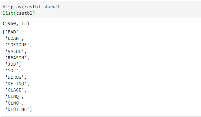

Displaying the Shape of the CAS Table:
- display(castbl.shape): This line utilizes the shape attribute of the CAS table object (castbl). The shape attribute typically returns a tuple representing the dimensions of the table, specifically the number of rows and columns. The display function is used here to showcase this information.
Obtaining a List of Column Names:
- list(castbl): The list function is applied to the CAS table (castbl). In Python, when you apply list to an object, it typically returns a list of its attributes or elements. In the context of a CAS table, this will return a list of column names present in the table

castbl.describe(include=['numeric', 'character'])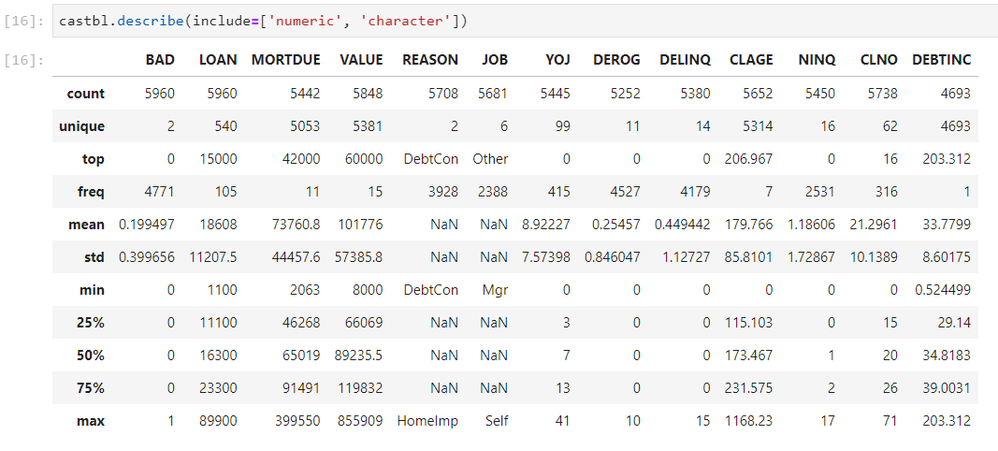

Impute Missing Values

conn.dataPreprocess.impute(
    table = indata,
    methodContinuous = 'MEDIAN',
    methodNominal    = 'MODE',
    inputs           = list(castbl)[1:],
    copyAllVars      = True,
    casOut           = dict(name = indata, replace = True)
)

using the impute method from the dataPreprocess module in the SWAT interface to perform data imputation on a SAS Viya server. Let's break down the components:

conn.dataPreprocess.impute(...):
- table = indata: Specifies the input table for the imputation operation. In this case, the variable indata is used, which was previously defined as a reference to the SAS Viya in-memory dataset.
- methodContinuous = 'MEDIAN': Sets the imputation method for continuous (numeric) variables to use the median. This means missing values in numeric columns will be replaced with the median of the respective column.
- methodNominal = 'MODE': Sets the imputation method for nominal (categorical) variables to use the mode. Missing values in categorical columns will be replaced with the mode of the respective column.
- inputs = list(castbl)[1:]: Specifies the columns on which imputation will be performed. The list(castbl) generates a list of column names from the CAS table castbl, and [1:] is a Python slice notation that includes all elements starting from the second element (index 1) onward. This effectively excludes the first element, which is often an identifier or target variable.
- copyAllVars = True: Indicates that all variables, including those not specified in the inputs, should be included in the output table.
- casOut = dict(name = indata, replace = True): Specifies the output table details. It sets the name of the output table as the same as the input (indata) and uses replace = True to replace the existing table if it already exists.

Create Variable Shortcuts

# Get variable info and types
colinfo = conn.table.columninfo(table=indata)['ColumnInfo']

# Target variable is the first variable
target = colinfo['Column'][0]

# Get all variables
inputs = list(colinfo['Column'][1:])
nominals = list(colinfo.query('Type=="varchar"')['Column'])

# Get only imputed variables
inputs = [k for k in inputs if 'IMP_' in k]
nominals = [k for k in nominals if 'IMP_' in k]
nominals = [target] + nominals

colinfo = conn.table.columninfo(table=indata)['ColumnInfo']: Retrieves information about the columns (variables) in the specified SAS Viya table (indata). The result is stored in the colinfo variable.
target = colinfo['Column'][0]: Extracts the name of the target variable, which is assumed to be the first variable in the table. This assumes that the target variable is located at index 0 in the column information.
inputs = list(colinfo['Column'][1:]): Creates a list of all variables (excluding the target variable) in the table by extracting the 'Column' information from the colinfo dataframe.
nominals = list(colinfo.query('Type=="varchar"')['Column']): Creates a list of variables that are of type 'varchar' (nominal/categorical) by querying the colinfo dataframe for columns with 'Type' equal to "varchar."
inputs = [k for k in inputs if 'IMP_' in k]: Filters the list of variables (inputs) to include only those that have 'IMP_' in their names. This assumes that imputed variables have names containing 'IMP_'.
nominals = [k for k in nominals if 'IMP_' in k]: Similarly filters the list of nominal variables (nominals) to include only those with 'IMP_' in their names.
nominals = [target] + nominals: Combines the target variable and the list of nominal variables (nominals) into a new list.

Split the Data into Training and Validation

conn.sampling.srs(
    table   = indata,
    samppct = 70,
    seed = 919,
    partind = True,
    output  = dict(casOut = dict(name = indata, replace = True),  copyVars = 'ALL')
)

conn.sampling.srs(...): Invokes the simple random sampling (SRS) method from the sampling module provided by the SWAT interface. This method is used for creating a random sample from the specified SAS Viya table.
table = indata: Specifies the input table (indata) from which the sample will be drawn.
samppct = 70: Sets the sampling percentage to 70%, indicating that the desired sample size is 70% of the total observations in the input table.
seed = 919: Specifies the seed for the random number generator. Using a seed ensures reproducibility, meaning that if the same seed is used, the same random sample will be generated.
partind = True: Includes a binary partition indicator variable in the output. This variable helps identify whether an observation is part of the sample (1) or not (0).
output = dict(casOut = dict(name = indata, replace = True), copyVars = 'ALL'): Specifies the output details. It creates a new SAS Viya table with the same name as the input (indata) and replaces it if it already exists (replace = True). The option copyVars = 'ALL' indicates that all variables from the input table should be included in the output.

Train Machine Learning Models

models = ['dt','rf','gbt']
actions = ['conn.decisionTree.dtreeTrain','conn.decisionTree.forestTrain','conn.decisionTree.gbtreeTrain']
def train_func(model):
    tmp_dict = dict(
        table    = dict(name = indata, where = '_PartInd_ = 1'),
        target   = target, 
        inputs   = inputs, 
        nominals = nominals,
        casOut   = dict(name = model+'_model', replace = True)
        
    )
    return tmp_dict

for i in list(range(len(models))):
    params = train_func(models[i])
    tmp_str = actions[i]+'(**params)'
    obj = eval(tmp_str)
    print(models[i])
    print(obj['OutputCasTables'])

models and actions lists: These lists contain model names (models) and corresponding action names (actions). The models are decision tree (dt), random forest (rf), and gradient boosting (gbt), and the actions are the corresponding Viya procedures for training these models.
train_func function: This function generates a dictionary of parameters for training a specific model. It includes details such as the input table, target variable, input variables, nominal variables, and the output table for the trained model.
for loop: Iterates over the list of models.
- params = train_func(models[i]): Calls the train_func function to get the parameters for the current model in the loop.
- tmp_str = actions[i]+'(**params)': Constructs a string that represents the Viya action for training the current model, including the parameters.
- obj = eval(tmp_str): Evaluates the string as a Python expression, effectively executing the Viya action for training the model. The result is stored in the obj variable.
- print(models[i]): Prints the current model name.
- print(obj['OutputCasTables']): Prints the output tables generated during the training process.

Models Scoring

models = ['dt','rf','gbt']
actions = ['conn.decisionTree.dtreeScore','conn.decisionTree.forestScore','conn.decisionTree.gbtreeScore']

# Create function to score a given model
def score_func(model):
    tmp_dict = dict(
        table    = dict(name = indata, where = '_PartInd_ = 0'),
        model = model+'_model',
        casout = dict(name=model+'_scored', replace=True),
        copyVars = target,
        encodename = True,
        assessonerow = True
    )
    return tmp_dict

# Loop over the models and actions
for i in list(range(len(models))):
    params = score_func(models[i])
    tmp_str = actions[i]+'(**params)'
    obj = eval(tmp_str)
    print(models[i])
    print(obj['ScoreInfo'].iloc[[2]])

models and actions lists: These lists contain model names (models) and corresponding action names (actions). The models are decision tree (dt), random forest (rf), and gradient boosting (gbt), and the actions are the corresponding Viya procedures for scoring data with these models.
score_func function: This function generates a dictionary of parameters for scoring data with a specific model. It includes details such as the input table, the trained model, the output table for the scored data, and other options.
for loop: Iterates over the list of models.
- params = score_func(models[i]): Calls the score_func function to get the parameters for scoring data with the current model in the loop.
- tmp_str = actions[i]+'(**params)': Constructs a string that represents the Viya action for scoring data with the current model, including the parameters.
- obj = eval(tmp_str): Evaluates the string as a Python expression, effectively executing the Viya action for scoring data with the model. The result is stored in the obj variable.
- print(models[i]): Prints the current model name.
- print(obj['ScoreInfo'].iloc[[2]]): Prints information about the scoring process, specifically extracting the third row of the 'ScoreInfo' output.

Model Assessment

# Create function to assess a given model
def assess_func(model):
    tmp_dict = dict(
        table = model+'_scored',
        inputs = 'P_'+target+'1',
        casout = dict(name=model+'_assess' ,replace=True),
        response = target,
        event = "1"
    )
    return tmp_dict

# Loop over the models
for i in list(range(len(models))):
    params = assess_func(models[i])
    obj = conn.percentile.assess(**params)
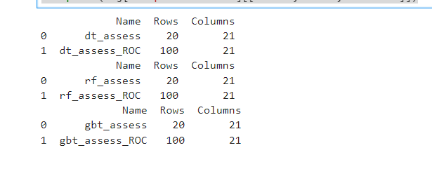
    print(obj['OutputCasTables'][['Name','Rows','Columns']])

assess_func function: This function generates a dictionary of parameters for assessing the performance of a specific model. It includes details such as the input table containing the scored data, the variable representing the predicted probabilities of the positive class ('P_'+target+'1'), the output table for assessment results, the response variable, and the event level for the response variable.
for loop: Iterates over the list of models.
- params = assess_func(models[i]): Calls the assess_func function to get the parameters for assessing the current model in the loop.
- obj = conn.percentile.assess(**params): Invokes the assess method from the percentile module provided by the SWAT interface. This method assesses the performance of a predictive model.
- print(obj['OutputCasTables'][['Name','Rows','Columns']]): Prints information about the output tables generated during the assessment process, including their names, number of rows, and number of columns.

# Create function to bring assess tables to the client
def assess_local_roc(model):
    castbl_obj = conn.CASTable(name = model+'_assess_ROC')
    local_tbl = castbl_obj.to_frame()
    local_tbl['Model'] = model
    return local_tbl

# Bring result tables to the client in a loop
df_assess = pd.DataFrame()
for i in list(range(len(models))):
    df_assess = pd.concat([df_assess, assess_local_roc(models[i])])

cutoff_index = round(df_assess['_Cutoff_'],2)==0.5
compare = df_assess[cutoff_index].reset_index(drop=True)
compare[['Model','_TP_','_FP_','_FN_','_TN_']]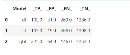

assess_local_roc function: This function takes a model name as input, creates a CAS table object (castbl_obj) associated with the ROC assessment results for that model, converts it to a Pandas DataFrame (local_tbl), adds a 'Model' column with the model name, and returns the resulting DataFrame.
for loop: Iterates over the list of models.
- df_assess = pd.concat([df_assess, assess_local_roc(models[i])]): Calls the assess_local_roc function for each model and concatenates the resulting DataFrames into the df_assess DataFrame.
cutoff_index = round(df_assess['_Cutoff_'], 2) == 0.5: Creates a boolean index based on the condition that the rounded 'Cutoff' column is equal to 0.5.
compare = df_assess[cutoff_index].reset_index(drop=True): Filters the df_assess DataFrame based on the condition, resets the index, and stores the result in the compare DataFrame.
compare[['Model', '_TP_', '_FP_', '_FN_', '_TN_']]: Extracts specific columns ('Model', 'TP', 'FP', 'FN', 'TN') from the compare DataFrame for comparison.

plt.figure(figsize=(8,8))
plt.plot()
models = list(df_assess.Model.unique())

# Iteratively add curves to the plot
for X in models:
    tmp = df_assess[df_assess['Model']==X]
    plt.plot(tmp['_FPR_'],tmp['_Sensitivity_'], label=X+' (C=%0.2f)'%tmp['_C_'].mean())

plt.xlabel('False Positive Rate', fontsize=15)
plt.ylabel('True Positive Rate', fontsize=15)
plt.legend(loc='lower right', fontsize=15)
plt.show()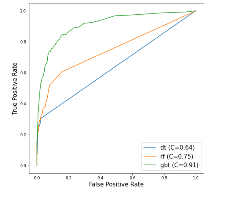

plt.figure(figsize=(8, 8)): Creates a new figure for the plot with a specified size of 8x8 inches.
plt.plot(): Initiates an empty plot.
models = list(df_assess.Model.unique()): Creates a list of unique model names based on the 'Model' column in the df_assess DataFrame.
for X in models:: Iterates over the list of unique model names.
- tmp = df_assess[df_assess['Model'] == X]: Filters the df_assess DataFrame to include only rows corresponding to the current model.
- plt.plot(tmp['_FPR_'], tmp['_Sensitivity_'], label=X + ' (C=%0.2f)' % tmp['_C_'].mean()): Plots the ROC curve for the current model. It uses the False Positive Rate ('_FPR_') on the x-axis and True Positive Rate ('_Sensitivity_') on the y-axis. The label includes the model name and the mean value of the threshold ('C') used for calculating sensitivity.
plt.xlabel('False Positive Rate', fontsize=15): Sets the x-axis label.
plt.ylabel('True Positive Rate', fontsize=15): Sets the y-axis label.
plt.legend(loc='lower right', fontsize=15): Adds a legend to the plot at the lower-right corner with the specified font size.
plt.show(): Displays the plot.

# Create function to bring assess results to the client
def assess_local_lift(model):
    castbl_obj = conn.CASTable(name = model+'_assess')
    local_tbl = castbl_obj.to_frame()
    local_tbl['Model'] = model
    return local_tbl

# Bring results to client in a loop
df_assess = pd.DataFrame()
for i in list(range(len(models))):
    df_assess = pd.concat([df_assess, assess_local_lift(models[i])])
    
plt.figure(figsize=(8,8))
plt.plot()
models = list(df_assess.Model.unique())
display(models)

# Iteratively add curves to the plot
for X in models:
    tmp = df_assess[df_assess['Model']==X]
    plt.plot(tmp['_Depth_'],tmp['_CumLift_'], label=X)

plt.xlabel('False Positive Rate', fontsize=15)
plt.ylabel('True Positive Rate', fontsize=15)
plt.legend(loc='upper right', fontsize=15)
plt.show()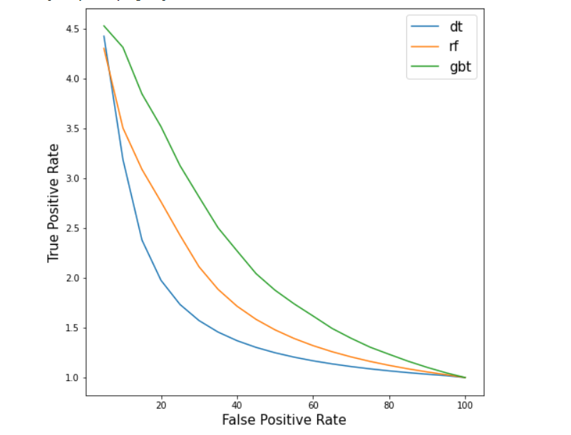

assess_local_lift function: This function takes a model name as input, creates a CAS table object (castbl_obj) associated with the assessment results for that model, converts it to a Pandas DataFrame (local_tbl), adds a 'Model' column with the model name, and returns the resulting DataFrame.
for loop: Iterates over the list of models.
- df_assess = pd.concat([df_assess, assess_local_lift(models[i])]): Calls the assess_local_lift function for each model and concatenates the resulting DataFrames into the df_assess DataFrame.
plt.figure(figsize=(8, 8)): Creates a new figure for the plot with a specified size of 8x8 inches.
plt.plot(): Initiates an empty plot.
models = list(df_assess.Model.unique()): Creates a list of unique model names based on the 'Model' column in the df_assess DataFrame.
for X in models:: Iterates over the list of unique model names.
- tmp = df_assess[df_assess['Model'] == X]: Filters the df_assess DataFrame to include only rows corresponding to the current model.
- plt.plot(tmp['_Depth_'], tmp['_CumLift_'], label=X): Plots the cumulative lift curve for the current model. It uses the 'Depth' column on the x-axis and 'CumLift' column on the y-axis.
plt.xlabel('Depth', fontsize=15): Sets the x-axis label.
plt.ylabel('Cumulative Lift', fontsize=15): Sets the y-axis label.
plt.legend(loc='upper right', fontsize=15): Adds a legend to the plot at the upper-right corner with the specified font size.
plt.show(): Displays the plot.

Save the Best Model

Add a CASlib:
```
conn.table.addCaslib(name="mycl", path=os.environ.get("HOME"), dataSource="PATH", activeOnAdd=False)
```
- This adds a CASlib named "mycl" pointing to the specified path, which is the user's home directory (os.environ.get("HOME")).
- The dataSource parameter indicates the type of the data source, which is set to "PATH" in this case.
- The activeOnAdd=False parameter indicates that the CASlib should not be set as the active CASlib upon addition.
Save a CAS Table (Model):
```
conn.table.save(caslib = 'mycl', table = dict(name = 'gbt_model'), name = 'best_model_gbt', replace = True)
```
- This saves the CAS table named 'gbt_model' in the CASlib 'mycl' with the name 'best_model_gbt'.
- The replace=True parameter indicates that if a table with the same name already exists, it should be replaced.
Save Model Attributes:

conn.table.attribute(caslib = 'CASUSER', table = 'gbt_model_attr', name = 'gbt_model', task='convert')
conn.table.save(caslib = 'mycl', table = 'gbt_model_attr', name = 'attr', replace = True)

The first line extracts attributes from the 'gbt_model_attr' CAS table, which is assumed to contain model attributes related to the 'gbt_model'.
The task='convert' parameter specifies that the attributes should be converted.
The second line saves the resulting attributes table in the 'mycl' CASlib with the name 'attr', replacing it if it already exists.