Machine Learning and Explainable AI in Forecasting - Part III

5 Likes

An Application for Explainable AI in Forecasting

Table of Content

Introduction

In this third part of our blog series we will show you how to create an easy to use application to explain Forecasting models on the fly. We will use SAS Visual Analytics, the Data Driven Content object and the SAS Job Execution Engine to create this application. Some things need to be done on the client side and some on the server side. We will explain each step on the client side and on the server side.

Example Report

Before we go deeper into the technical detail of each of the different steps, let’s have a look at how a typical report that uses our application would look like.

(view in My Videos)

As we see from the video this interactive report would be a tool that would be used by reporting analysts, planners, management and other business personas to get a deep insight into the drivers that have an impact on the final forecasts.

Note: The example report shows forecasts where historical data is also available but it would work exactly the same with no limitations for future forecasts as well since the method is focusing on explaining the prediction of a machine learning model without taking actual data into consideration.

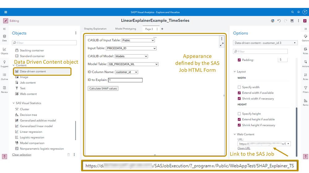
Now let’s have a look at how you can build a similar report and tailor it to the business needs of your organisation.

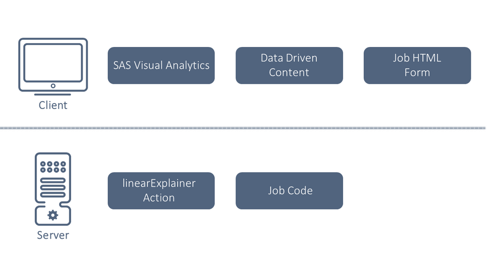
Client

Let's first take a look at SAS Visual Analytics. Within SAS Visual Analytics there is a huge selection of different visualization objects available to create reports, insights or analytical models. The Data Driven Content object let s you add customized visualizations and run custom code. In the screenshot below you can see where to select this object on the left hand side of SAS Visual Analytics. In the middle you can see a HTML form that let you select the settings to run the code on the server side. The content of the Data Driven Conent object is included by the URL property of this object shown on the right hand side of the screenshot.

The HTML torm enables the user to select and enter/autofill all the settings that are needed to run the job code. The settings are selected through pre-populated dropdowns and entered/autofilled in an input field. In total the following information is needed: The CAS-Library (1 & 3) in which the Input table and the Model table are located, the Input table (2) and the Model table (4) that are being used, the ID column (5) of the Input table and the value of the ID (6).

The implementation of this application has three major parts:

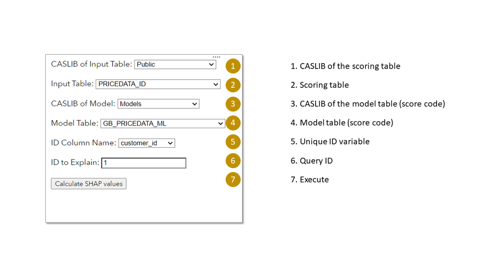
For the pre-populated dropdowns (1-5) we call the casManagement APIs
To preserve automated actions on objects (autofill the query ID) we need to receive the data of SAS Visual Analytics
Executing the SAS Job

1. Calling the casManagement API

The API calls are done relative to the winows.origin property of the server so that the code should run dynamically in any Viya installation. The calls are made utilizing the fetch function:

fetch(
        window.origin +
          '/casManagement/providers/cas/sources/cas-shared-default/children?limit=100&sortBy=name%3Aascending&start=0',
        {
          // mode: 'no-cors',
          method: 'GET',
          headers: {
            Accept: 'application/json',
          },
        }
      ).then((response) => {
        if (response.ok) {
            // Do stuff here
        }))

As the pre-loaded dropdowns depend on the users' selection the calls are chained and when one of the parent value changes the child data is refreshed as well.

2. Receiving Data from SAS Visual Analytics (VA)

In our application we would like to give the user the option to select a specific observation through a line chart and autofill the "ID to Explain" field (6). In order to achieve automated actions between standard visualization objects and the data driven content object, the object needs to receive data from VA. The SAS VA Messaging Uti allows you to receive the data. The implementation is simple as the ID field is unique.

function onDataReceived(resultData) {
        ID.value = resultData.data[0];
      }

va.messagingUtil.setOnDataReceivedCallback(onDataReceived);

3. Executing the SAS Job

Once the user clicks on the Calculate SHAP values button (7) a spinner overlay is added (to give a visual indication that the job is running) and the SAS Job gets called with all the values the user provided in the form:

fetch(jeeURI, {
	method: 'GET',
	})
    .then((resp) => {
    	console.log('Response');
        SPINNER.style.display = 'none';
        FORM.style.display = 'block';
    })
    .then((body) => {
    	console.log('Success');
    })
    .catch((error) => {
    	console.log('Error');
    });
});

On a response the spinner is overlay is hidden again and the user can interact with the form again. This allows the

user, after an initial set up of the main parameters (1-5), to quickly iterate through more IDs.

Note: The code above is written in Javascript and included inline in the HTML form.

Server

As already described in the section above the following values are captured by the client:

Variable name in the code	Description
caslib_ds	CASLIB of the scoring table
name_ds	Scoring table
caslib_m	CASLIB of the model table (score code)
name_m	Model table (score code)
id_name	Unique ID variable
id	Query ID

The first step loads the model into memory, to make sure that it is available for execution. You can load data into memory with proc casutil.

After the model is loaded, the model's input and output information is extracted from the model to reduce user inputs:

proc astore;
    ods output InputVariables=work.inputs;
	ods output OutputVariables=work.outputs;
	describe rstore=&caslib_m..&name_m.;
run;

The query table will be create based on the id variable and it's value:

data casuser.query;
	set &caslib_ds..&name_ds.(where=(&id_name=&id));
run;

After all necessary information is available, a CASL program is generated and stored in a .sas-program based on the information collected above. The program needs to be generated on the fly because every model can have different predictor and outcome variables. In addition, a model can have interval and nominal predictors. In this case the syntax of the code will differ slightly.

Here are two examples of the generated code. One for the global explanation of Forecasting models and one for the local explanation of Forecasting models. The theory of these methods is explained in the second part of our blog series.

Global Explanation Example Code

In this example the preset parameter is set to 'GlobalReg' and the dataGeneration method is set to 'None', which would be the default in this case. Details can be found here.

explainModel.linearExplainer result=globr / table = {name='PRICEDATA_ID', caslib='PUBLIC'}
 query = {name='QUERY', caslib='CASUSER'}
 modelTable = {name='GB_PRICEDATA_MODEL_ID', caslib='MODELS'}
 modelTableType = 'ASTORE'
 predictedTarget = 'P_sale'
 seed=1234
 preset = 'GlobalReg'
 dataGeneration = {method='None'}
inputs= {{name = "sale_lag3"},
{name = "sale_lag2"},
{name = "sale_lag1"},
{name = "discount"},
{name = "price"}}
;run;
send_response({gr=globr['ParameterEstimates']});run;

The generated program will be referenced by the filename pgm_g and executed by the runCASL action:

proc cas;
	session casauto;
	loadactionset "explainModel";
	loadactionset "sccasl";
	source pgm_g;
	%include pgm_g;
	endsource;
	run;
	sccasl.runCASL result=r / code=pgm_g;
	run;
	describe r;
	param_est=findtable(r);
	saveresult param_est dataout=work.parameterEstimates;
quit;

Local Explanation Example Code

We slightly change the parameters to perform a local explanation:

explainModel.linearExplainer result=shapr / table = {name='PRICEDATA_ID', caslib='PUBLIC'}
 query = {name='QUERY', caslib='CASUSER'}
 modelTable = {name='GB_PRICEDATA_MODEL_ID', caslib='MODELS'}
 modelTableType = 'ASTORE'
 predictedTarget = 'P_sale'
 seed =1234
 preset = 'KERNELSHAP'
 dataGeneration = {method='None'}
inputs= {{name = "sale_lag3"},
{name = "sale_lag2"},
{name = "sale_lag1"},
{name = "discount"},
{name = "price"}}
;run;
send_response({sr=shapr['ParameterEstimates']});run;

The result tables will be stored/refreshed to CAS and can be accessed and visualized by the SAS Visual Analytics report everytime a user clicks the "Execute" button.

Conclusion

This concludes our series of articles. We hope you enjoyed reading them and found them useful. We've touched upon many different topics so don't despair if some areas are still unclear - this is perfectly normal. What we hope you take out from these articles is a good understanding of Machine Learning techniques in forecasting and how you can cleverly apply existing state-of-the-art techniques to explain your forecasts. In the last article, we've also shown how you can create a custom application to dynamically run explainability techniques on the fly using SAS Viya's powerful capabilities. The final application provides strong insights in your forecasts and is extremely easy to use by any business stakeholder. As a last thought we want to mention that explainability in forecasting has attracted the attention of many researchers recently and we expect a lot of new exciting developments in this area. As always, we'll make sure to keep you updated!