Machine Learning and Explainable AI in Forecasting - Part II

3 Likes

Explainability Methods in Forecasting

Table of Content

Introduction

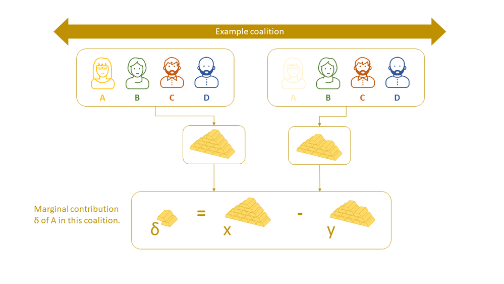
In this second part of our blog series we focus on SHAP[1] as local explanation method and how to apply this method to the ABT table we created from the time series data. As we mentioned in part I the challenge we are facing is that this method works well when the variables we are using are independent from each other, so we have to find a way to adapt our methodology to overcome this issue.

But before we start, let's give you a short introduction into Shapley Values.

What are Shapley Values?

The concept of Shapley Values came from economists[2] for game theory. They tried to solve the problem of award distribution among multiple team members.

How to fairly attribute member's contribution? The solution by Lloyd Shapley satisfies the following properties:

EFFICIENCY: All individual awards should add up to the total earning
DUMMY: If including an individual brings no additional earning in any situation, then this individual should receive zero award
SYMMETRY: If including two individuals add the same amount of additional earnings, then they should receive the same award
ADDITIVITY: If including individual A inceases the earning by the same amount of two other individuals B and C, then A should receive the sum of B's and C's award.

The Shapley Value is the ONLY solution that satisfies all constraints! It is based on a weighted marginal contribution of a member among all possible coalitions.

But wait what is a coalition and what is a marginal contribution?

What would be the weighted marginal contribution among all possible coalitions? Here is an example Shapley Value for member A:

Written as formula:

See: https://christophm.github.io/interpretable-ml-book/shapley.html

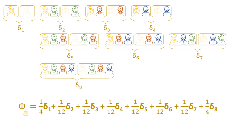
In the formula above, p is the total number of members and S is the number of members in the coalition excluding the member of interest.

The weight is inversely proportional to the size of a coalition “group” where each “group” includes all coalitions with the same number of members.

So, in our example above we have 4 groups:

Group 1: Adding 0 other person, size 1
Group 2: Adding 1 other person, size 3
Group 3: Adding 2 people, size 3
Group 4: Adding 3 people, size 1

Each group ends up in having the same total weight of 1/4 and all weights add up to 1.

This approach can be transferred to explain the prediction for a (local) observation. Each feature value of the observation is a member in a game where the prediction is the award.

The calculation of Shapley Values is computationally expensive as it requires the evaluation of the model with all possible coalitions/combinations of features. There are faster approximation methods available, like SHAP[1].

This SHAP method is implemented in the SAS action linearExplainer which is one action of the Explain Model action set.

A good explanation of the SHAP method can be found in the book Interpretable Machine Learning.

In the next section we will explain how to adapt the linearExplainer action for time series data.

Using the linearExplainer Action for Time Series Data

The standard KERNELSHAP preset implementation of the SAS action is following these steps:

Pick a single observation (query)
Generate random observations by sampling from each variable's distribution separately
Apply the model score code that was generated by a previous step to the new observations
Weight the observations based on their coalitions
Run a weighted linear regression on model's prediction
Interpret the linear regression model coefficients

Because of the way we built our analytical base table (ABT) - transferring it from transactional to one row per subject - our features are not independent from each other. For details, please refer to part I of our blog series. When we would apply step 2 - generating random observations - the dependency among the features would get lost.

To preserve the dependency structure, it is possible to suppress the random sampling process 😊. Here is an example code:

proc cas;
explainModel.linearExplainer result=shapr / table = {name='PRICEDATA_ID', caslib='PUBLIC'}
 query = {name='QUERY', caslib='CASUSER'}
 modelTable = {name='GB_PRICEDATA_MODEL_ID', caslib='MODELS'}
 modelTableType = 'ASTORE'
 predictedTarget = 'P_sale'
 seed =1234
 preset = 'KERNELSHAP'
 dataGeneration = {method='None'}
inputs= {{name = "sale_lag3"},
{name = "sale_lag2"},
{name = "sale_lag1"},
{name = "discount"},
{name = "price"}}
;
run;

So, by adding the line of code "dataGeneration = {method='None'}", random sampling will be suppressed and the model's score code will be applied to the original observations.

This preserves the feature dependencies and let you explain the prediction of machine learning models like Gradient Boosting or other tree based algorithms like LightGBM in our Forecasting case.

However, please note that

the accuracy depends on how well the original data cover the coalitions,
the Shapley values of highly correlated features may bleed into each other,
this method can be seen as approximation of the Shapley coalition/cohort values in [3].

Note: If you are interested in a global explanation of your machine learning model for time series data, you can just adapt the preset parameter to 'GLOBALREG' to create a surrogate model for a global explanation of your model.

In our third and last part of this blog series, we will show how to explain forecasting models globally and locally in an application.

See you in part III!

References

[1] Lundberg, S. M., and Lee, S.-I. (2017). “A Unified Approach to Interpreting Model Predictions.” In A...

[2] Shapley, Lloyd S. “A value for n-person games.” Contributions to the Theory of Games 2.28 (1953): 307-317

[3] Mase et al. 2019 "Explaining black box decisions by Shapley cohort refinement"