- Home
- /
- SAS Communities Library
- /
- Incorporate prior knowledge (code a Bayesian prior for Proc BGLIMM)
- RSS Feed
- Mark as New
- Mark as Read
- Bookmark
- Subscribe
- Printer Friendly Page
- Report Inappropriate Content
Incorporate prior knowledge (code a Bayesian prior for Proc BGLIMM)
- Article History
- RSS Feed
- Mark as New
- Mark as Read
- Bookmark
- Subscribe
- Printer Friendly Page
- Report Inappropriate Content
Executive summary
Classical statistics and Bayesian models usually produce similar outcomes. Incorporating expert-informed prior knowledge through a Bayesian model gives the model a new dimension.
Introduction
Researchers who rely on designed experiments often rely on Generalized Linear Models (GzLMMs) including ANOVA, mixed models and logistic regressions. These models are often sufficient or superior to alternatives. More recently, Bayesian models have gained traction in part due to their ability to incorporate expert knowledge.
In this article, I share a data set ("luffa_day1", attached), compare a generalized linear model (Proc Glimmix) to a Bayesian model (Proc BGLIMM), with a non-informative prior. I also code another data set "prior" that I use to input an informed prior into the Proc BGLIMM model. This example demonstrates the ability to incorporate prior knowledge through an informed Bayesian prior.
Data set, assumptions and model considerations
Design and setup
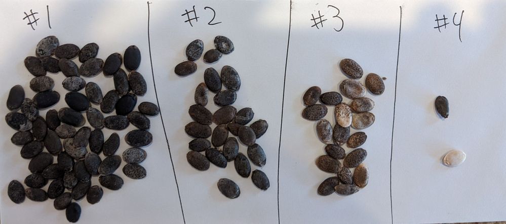
The Luffa_Day1 data represents an overnight imbibition test of Luffa aegyptiaca seeds. Seeds of this gourd species are hard and resistant to absorbing water (imbibition). The lot from which the data was generated showed a lot of variability in seed maturity (Grade_1 = best through Grade_4 = worst). Each Lot represents a container (plot) completely randomized. The lots contains 10 subplots as a 2*5 matrix of row (1 or 2) by column (1 through 5) representing the spatial distribution of subplots within each lot.
The 16 lots were stratified a 2*4 design as Top = 1 (on, sealed into a humid chamber) and Top = 0 (off, open air), and 4 levels of Water applied to paper towel media (93.6 to 138 mm). There were two technical replicates per treatment. BBCH_00 represents hard seed (not imbibed), and BBCH_01 and BBCH_03 represent increasing levels of imbibition. Prop_Dry was calculated as BBCH_00 divided by Count, the number of seeds in the subplot. Total represents the total seeds allocated to the lot.
Model and assumptions
I imported the data attached into my "Casuser" caslib and named the table "Luffa_Day1" First thing I wanted to do was standardize continuous input variables, outputting the table as "luffa2":
proc stdize data=casuser.Luffa_day1 out= casuser.luffa2;
var Water Grade_1;
run;
I modeled Prop_dry as the response variable, in each case assuming a normal, continuous distribution of data. Poisson, binary or binomial distributions should also considered.
The model considered explanatory variables of Water (continuous parameter), Grade_1 (continuous parameter) and Top (binary parameter). Interaction effects (e.g. Water*Top) may also be considered.
The models consider each explanatory variable as a fixed effect. The Procedures used support mixed parameterizations (random statements) and some effects could be considered random.
Classical statistical model versus Bayesian
Proc GLIMMIX (Generalized Linear Mixed model) and Proc BGLIMM (Bayesian Generalized Linear Mixed model) have similar encodings, allowing easy re-coding in one versus another.
proc bglimm data= casuser.luffa2 nmc=100000 thin=2 seed=806 plots=all;
	class Lot Top;
	model Prop_Dry=Water Top Grade_1/ dist=normal link=identity cprior=normal(var=1e4);
   ESTIMATE 'Dry Open Air' intercept 1 water -1 top 0 1;
   ESTIMATE 'Wet Open Air' intercept 1  water 1 top 0 1;
   ESTIMATE 'Dry Humid Chamber' intercept 1 water -1 top 1 0;
   ESTIMATE 'Wet Humid Chamber' intercept 1  water 1 top 1 0;
run;

proc glimmix data= casuser.luffa2 plots=pearsonpanel;
	class Lot Top;
	model Prop_Dry=Water Top Grade_1/ dist=normal link=identity s cl ;
   ESTIMATE 'Dry Open Air' intercept 1 water -1 top 0 1 /cl;
   ESTIMATE 'Wet Open Air' intercept 1  water 1 top 0 1 /cl;
   ESTIMATE 'Dry Humid Chamber' intercept 1 water -1 top 1 0 /cl;
   ESTIMATE 'Wet Humid Chamber' intercept 1  water 1 top 1 0 /cl;
run;
The default model selections (assuming a normal distribution and identity links) are included. The differences include:
- options within the Procs (see documentation for details)
- the cprior option in the BGLIMM model statement (this is the mechanism to incorporate prior knowledge, if available), and
- the need to explicitly request confidence limits (cl) for GLIMMIX estimate statements (BGLIMM provides comparable 95% HPD intervals by default).
The "cprior=normal(var=1e4)" is a noninformative prior, which means, like classical statistical models, parameter estimates are not anchored to a predilected value.
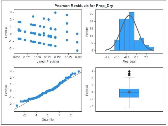
The output includes GzLMM Pearson residual and Bayesian diagnostics plots:
Whereas the GzLMM models adhere to assumptions of normality, independence and homoskedasticity poorly to moderately, the Bayesian diagnostics are textbook good: good mixing without any wave patterns (upper panel) and practically chain autocorrelation. Confidence that the model bears out its assumptions is a valid reason to choose one model over another.
At the end of the day, the models produced similar results. The parameter estimates were of a similar direction and magnitude, though the confidence limits (GzLMM) were slightly smaller than HPD intervals (Bayesian), which means that p-values for the GzLMM were smaller than for Bayesian models. This p-value assessment isn't a great way to judge a model (and the difference wasn't that big anyway), and in any case the two models show similar results:
Why and how to incorporate prior knowledge
Reasons to incorporate prior knowledge include:
- There's data from another experiment that can't be directly combined with this one
- This data set has limited data that can be augmented by expert judgment
- To assess the reasonableness of the current data, given what was known previously
How to turn prior knowledge into a numerical prior
In the case of this experiment, I hypothesized that Grade 1 seeds will imbibe more slowly than others. This is because I observed these seeds had a thick coat and apparently more cuticular wax than some of the lesser grades. Without any prior germination data, I hypothesized that 1 unit increase in Grade 1 (this is based on standardized data, so 1 standard deviation or 34% increase) results in proportion 0.1 fewer seeds imbibed overnight.
Based on my observations, I was confident that 3-4 more Grade 1 seeds in a batch of 10 would result in an additional 1/10th of the seeds delaying inhibition, so the variance I assigned to this prior mean (0.1) was a low number (0.0001). If I was less confident, my variance would have been higher, which would have made my prior count for less when the final posterior distribution was sampled. One critique of informed Bayesian priors is that while experts can often do a good job assessing the mean, naming variance can be more difficult. One recommendation is to try different variances to see what effect that has on the model.
Coding a prior for Proc BGLIMM
You need two lines, mean and cov, with the variable name in each row for which you can assign interactions and covariances with other variables. I did not assume anything for the mean or covariance relationship with intercept or water, only grade_1. Here it is in code
/*For every additional standard deviation in grade 1 seed, I expect that seed (1/10 =.1) not to imbibe*/
/*I am quite certain about this assessment (higher Cov = less certainty)*/
data prior;
input _Type_$ _Name_$ Intercept Water Grade_1;
datalines;
Mean Grade_1 0 0 .1
Cov Grade_1 0 0 .0001
;
That's the prior data table. Now, we will read it into the model in the cprior option of the model statement ("input=prior" because 'prior' was the name of the data set representing the prior):
proc bglimm data= casuser.luffa2 nmc=100000 thin=3 nbi=1000 seed=806 plots=all ;
	class Lot Top;
	model Prop_Dry=Water Top Grade_1 / dist=normal link=identity cprior=normal(input=prior);
   ESTIMATE 'Dry Open Air' intercept 1 water -1 top 0 1;
   ESTIMATE 'Wet Open Air' intercept 1  water 1 top 0 1;
   ESTIMATE 'Dry Humid Chamber' intercept 1 water -1 top 1 0;
   ESTIMATE 'Wet Humid Chamber' intercept 1  water 1 top 1 0;
run;
The results of incorporating the prior
First, the diagnostics looked very similar to the one in the previous example (not shown) including that its lower left panel (the histogram) also maintained a well-defined peak. This was a relief because priors that are strong (low variance) and oddball [distant from the present data (likelihood)] can create a bimodal posterior distribution, which wouldn't make sense. In other cases, strong priors can increase the standard deviation of estimates, which can be good considering model generalizability, or bad considering fit.
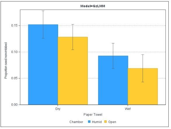
The outcome showed a different direction of effect for whether the top was sealed to create a humid chamber, and dampened the estimated effect of paper towel wetness. In other words, the prior changed the results in a stark and meaningful way.
While there aren't instances of particular treatments HPD intervals (represented by error bars) not overlapping (and likely not significantly different at p<0.05), you can still interpret the relative level and magnitude of effect each treatment has on the seedlings. For example, it would be very surprising if there were 2/10 seeds non-imbibed in the wet humid chamber condition, but not so much in the dry, open environment. In this way, we have incorporated prior knowledge that changed the course of our statistical assessment, and provided additional value to the research.
Conclusions
GzLMMs and Bayesian model outcomes are often comparable, especially when there is no prior information available. When prior information is available, it is always a good idea to try to fold that into a model somehow.
In practice and even when data is limited, weak Bayesian priors often sway the model too little to make up for the trouble of their construction, diagnostics and defense. Sources of prior information can alternatively be coded in classical statistics or machine learning contexts such as through new feature inclusion or loss functions.
Bayesian statistics do have several advantages including better p-value interpretability and (as we saw here) allowing us to relax some assumptions in the face of hardened real-world data. Bayesian priors are a battle-tested way to deliver expert insights faster.
April 27 – 30 | Gaylord Texan | Grapevine, Texas
Registration is open
Walk in ready to learn. Walk out ready to deliver. This is the data and AI conference you can't afford to miss.
Register now and lock in 2025 pricing—just $495!
SAS AI and Machine Learning Courses
The rapid growth of AI technologies is driving an AI skills gap and demand for AI talent. Ready to grow your AI literacy? SAS offers free ways to get started for beginners, business leaders, and analytics professionals of all skill levels. Your future self will thank you.


