Implementing Column Generation using SAS Optimization in SAS Viya

[#1]

In this article, I solve the Cutting Stock Problem by implementing a Column Generation algorithm using the action set Optimization in SAS Viya.

Column Generation methods are used successfully in large-scale Mathematical Optimization problems that occur frequently in the airlines, telecommunications, logistics and other industries.

These large-scale problems have thousands of variables (or columns) and enumerating them explicitly is not possible. By using the dual information that is obtained solving the master problem, new variables (or columns) are priced out (or generated). Other examples of column generations methods are the Dantzig-Wolfe Decomposition principle and Branch and Price. See my article on Implementing Column Generation using SAS Optimization Decomposition to Solve Large-Scale Problems about the SAS Decomposition Algorithm, which is based in the Dantzig-Wolfe Decomposition principle and can be implemented to take advantage of the distributed, cloud-based computational environment that SAS Viya provides.

According to George Nemhauser: “Column generation refers to linear programming (LP) algorithms designed to solve problems in which there are a huge number of variables compared to the number of constraints and the simplex algorithm step of determining whether the current basic solution is optimal or finding a variable to enter the basis is done by solving an optimization problem rather than by enumeration”

A quick search on the INFORMS journals for "Column Generation" resulted in 9 articles published between July and August 2019, in the journals Operations Research, Transportation Science, INFORMS Journal on Computing, INFORMS Journal on Optimization. The search returned 851 articles published from 1968 to August 2019. Searching for "Column Generation" in Google shows articles in the Journal of Artificial Intelligence Research, European Journal of Operational Research, IEEE Xplore Digital Library, etc.

Cutting Stock Problem

The Cutting Stock problem and its mathematical formulation are easy to understand. The problem to solve is: “how to cut a log into smaller stocks of different widths and demands” and it can be solved using Column Generation algorithms.

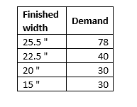
As an example, let’s assume that we want to cut a 91-inch log into smaller stocks of different widths and demands as shown in this table:

One way to cut the 91” log would be cutting 3 stocks of 25.5” finished-with and the resulting waste would be 14.5”. Another way would be cutting four stocks of 20” finished-width and the resulting waste would be 11”. There are many ways to cut the 91-inch log, some of those ways (or patterns) could result in a considerable amount of waste. The idea is to use the least possible number of 91” logs with minimum waste while satisfying the demand of finished-width logs.

Imagine a logistics company that has many depots, at each depot there are several trailer-size loads that need to be moved to different depots. Moreover, the pick-up and delivery of those trailer-size loads must occur during a specific time-window. The objective then would be to find the minimum number of routes that efficiently connect those depots to timely pick up/distribute the trailer-size loads.

Now imagine that you work for a Fortune 100 Airline company and you must develop its flight schedules. One would like to find the minimum number of flights that connect the cities where that airline flies while satisfying customer demand for all legs in all flights (also within specific time-windows).

There are many ways to cut the 91” log, many ways to create the routes that connect the depots, many ways to develop flight schedules, and Column Generation algorithms are used to solve these problems.

In this article, I will use a very simple version of the Cutting Stock problem. Still, the mathematical formulation and the code provided illustrate the concepts and can be used as basis for more complex problems.

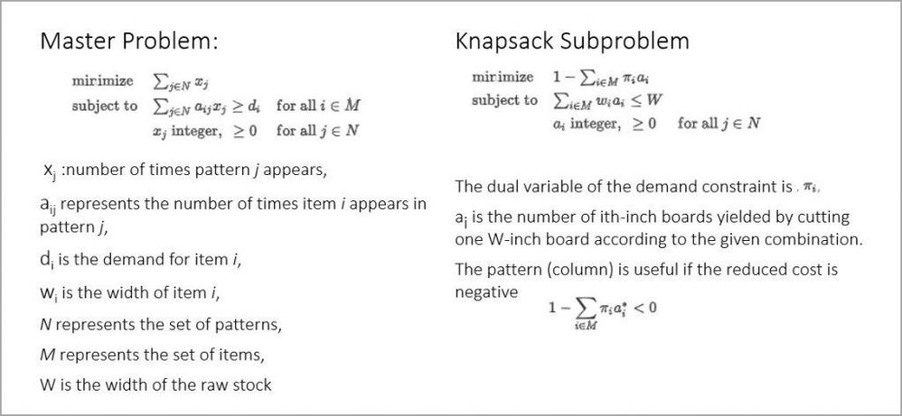
Mathematical Formulation of the Cutting Stock Problem

Select any image to see a larger version.
Mobile users: To view the images, select the "Full" version at the bottom of the page.

Solving the Cutting Stock Problem Using SAS Optimization in Viya

SAS Optimization is the general-purpose optimization product that takes advantage of the distributed, cloud-based computational environment that SAS Viya provides. L arge-scale problems benefit from running in a VIYA environment and their run time can be further shortened by parallelizing their subproblems.

SAS Optimization has these solvers: LP, MILP, QP, NLP, CLP, LSO and Network. Which are called thru Action Sets (Optimization and Network Optimization), whose actions can be submitted thru a variety of clients such as PROC CAS via SAS Studio, or through similar syntax in Python, Java, or Lua.

In this article, I will use the runOptmodel action in the Optimization Action Set to submit PROC OPTMODEL code to the CAS server.  

Pseudo-Code to Solve the Cutting Stock Problem

Steps to generate the patterns and solve the cutting stock problem:

1. Initialize LP with a set of trivial patterns N.
2. Solve the Master problem using the LP solver.
   • The LP solution are the x_j (number of times pattern j will be used) and the dual values of each constraint
3. Solve the Subproblem: Minimize the reduced cost using a knapsack solver
   • Results will indicate which new column(s) to add to the LP
   • If the reduced cost is negative add column(s) to LP.
4. Repeat steps 2 and 3 until there are no more negative reduced cost patterns.
5. Use the latest LP solution as warm-start for the MILP solver

Code

*How to solve the Cutting Stock Problem using Column Generation techniques
with SAS Optimization in Viya 3.4;

cas mySession1d sessopts=(caslib=CASUSER timeout=1800 locale="en_US");
libname CASUSER cas caslib=CASUSER ;

data CASUSER.indata;
   input type demand width;
   datalines;
1  78 25.5
2  40 22.5
3  30 20
4  30 15
;

* Using SAS macros facilitates the use of parameters that can be changed easily, as in this example the variable capacity;
%macro csp(capacity);

/* In this example we use the Action Set Optimization */
proc cas;
loadactionset "Optimization";
source pgm;
   /* declare parameters and sets */
   num capacity = &capacity;
   set ITEMS;
   num demand {ITEMS};
   num width  {ITEMS};
   num num_patterns init card(ITEMS);
   set PATTERNS = 1..num_patterns;
   num a {ITEMS, PATTERNS};
   num c {ITEMS} init 0;  /* It will hold the dual variables of the demand constraint */
   num epsilon = 1E-6;

   /*  read input data */
   read data CASUSER.indata into ITEMS=[type] demand width;

   /* generate trivial initial columns */
   for {i in ITEMS, j in PATTERNS}
      a[i,j] = (if (i = j) then floor(capacity/width[i]) else 0);

   /* define master problem */
   var x {PATTERNS} >= 0 integer;
   minimize NumberOfRaws = sum {j in PATTERNS} x[j];
   con demand_con {i in ITEMS}:
      sum {j in PATTERNS} a[i,j] * x[j] >= demand[i];	
   problem Master include x NumberOfRaws demand_con;

   /* define column generation subproblem */
   var y {ITEMS} >= 0 integer;
   maximize KnapsackObjective = sum {i in ITEMS} c[i] * y[i];
   con knapsack_con:
      sum {i in ITEMS} width[i] * y[i] <= capacity; 
   problem Knapsack include y KnapsackObjective knapsack_con;
   
   /* main loop */ 
   do while (1); 
   /* master problem */ 
   /* minimize sum_j x[j] subj. to sum_j a[i,j] * x[j] >= demand[i]
                  x[j] >= 0 and integer */
      use problem Master;
      put "solve master problem";
      solve with lp relaxint /
         presolver=none solver=ps basis=warmstart printfreq=1;
      print "Master Problem Solution";	
      print x;
      print demand_con.dual;

      for {i in ITEMS} c[i] = demand_con[i].dual;

      /* knapsack problem */
      /* maximize sum_i c[i] * y[i]
         subj. to sum_i width[i] * y[i] <= capacity 
                  y[i] >= 0 and integer */
      use problem Knapsack;
      put "solve column generation subproblem";
      print "Column Generation subproblem solution: Finding new pattern";
      solve with milp / printfreq=0;
      for {i in ITEMS} y[i] = round(y[i]);
	 
      print y;
      print KnapsackObjective;

      if KnapsackObjective <= 1 + epsilon then leave; 
         
      /* include new pattern */ 
      num_patterns = num_patterns + 1; 
      for {i in ITEMS} a[i,num_patterns] = y[i]; 
   end; 
     
   /* solve IP, using rounded-up LP solution as warm start */ 
   use problem Master; 
   for {j in PATTERNS} x[j] = ceil(x[j].sol); 
   put "solve (restricted) master problem as IP"; 
   solve with milp / primalin; 

   /* cleanup solution and save to output data set */ 
   for {j in PATTERNS} x[j] = round(x[j].sol); 
   create data solution from [pattern]={j in PATTERNS: x[j] > 0}
      raws=x {i in ITEMS} <col('i'||i)=a[i,j]>;

   endsource;
	
  optimization.runOptmodel / code=pgm;

  run;
quit;

%mend csp;

%csp(91);

Results and Analysis

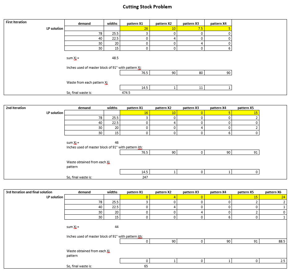
The Excel table below shows the results. For this simple problem, there are three iterations of the main loop that solves the LP Master and then the Knapsack subproblem until there are no more negative reduced cost patterns.

The first iteration starts with a feasible set of four patterns, the Master objective function is 48.5 which indicates that the pattern X1 is used 26 times, the pattern X2 is used 10 times, the pattern X3 used 7.5 times (non-integer!) and the pattern X4 is used 5 times with a final waste from using these four patterns of 474.5. The subproblem finds a new pattern X5 = (2,0,2,0).

The second iteration starts with 5 patterns, the Master objective function is 46 and the final waste from using these five patterns is 247. The subproblem finds a new pattern X6 = (2,1,0,1).

The third iteration starts with 6 patterns, the Master objective function is 44, and the final waste from using these six patterns is 65. In the subproblem, the reduced costs are positive which indicates that there are not new patterns that would improve the solution and the while loop ends.

The integer solution found is the same as the one found in the last LP. One should use pattern X2 four times, pattern X4 once, pattern X5 15 times and pattern X6 24 times, for a total of using 44 91-in logs.

If you wish, you could run the SAS code provided in this article and analyze the logs which show in detail information on the iterations.  

Conclusion

Implementing Column Generation algorithms using SAS Optimization allows for a clear Master and Subproblems definitions. In this article, the Subproblem is very simple and in “real-world” situations the Subproblem is more complex. Using SAS Optimization, one can declare and solve complex subproblems while clearly implementing the iterations between Master and Subproblem.  

References

Dantzig, G. B., and Wolfe, P. (1960). “Decomposition Principle for Linear Programs.” Operations Research 8:101–111.

Barnhart, C., Johnson, E. L., Nemhauser, G. L., Savelsbergh, M. W. P., and Vance, P. H. (1998). “Branch-and-Price: Column Generation for Solving Huge Integer Programs.” Operations Research 46:316–329.

Erwin Walraven, Matthijs T. J. Spaan, "Column Generation Algorithms for Constrained POMDPs," JAIR, Vol 68

A. Pessoa, R. Sadykov , E. Uchoa, F. Vanderbeck, "Automation and Combination of Linear-Programming Based Stabilization Techniques in Column Generatio... INFORMS journal on Computing, Vol. 30, No. 2

Capelle, Thomas & Cortés, Cristián E. & Gendreau, Michel & Rey, Pablo A. & Rousseau, Louis-Martin, "A column generation approach for location-routing problems with pickup and delivery," European Journal of Operational Research, Elsevier, vol. 272(1), pages 121-131.

Liyuan Zhang, Zhiguo Gui, Jie Yang, Pengcheng Zhang, "A Column Generation Approach Based on Region Growth," IEEE Access, Vol. 7

Qie He, Stefan Irnich, Yongjia Song, "Branch-and-Cut-and-Price for the Vehicle Routing Problem with Time Windows and Convex Node Costs"

Vahid Zeighami, François Soumis, "Combining Benders’ Decomposition and Column Generation for Integrated Crew Pairing and Personalized... Transportation Science

Maxence Delorme, Manuel Iori, "Enhanced Pseudo-polynomial Formulations for Bin Packing and Cutting Stock Problems," INFORMS Journal on Computing

To Try SAS Optimization

If you’d like to find out more, visit the SAS Optimization site which has instructions on how to try the software for free.