- Home
- /
- SAS Communities Library
- /
- How to Develop SAS Code to Train a Deep Learning Model for Image Class...
- RSS Feed
- Mark as New
- Mark as Read
- Bookmark
- Subscribe
- Printer Friendly Page
- Report Inappropriate Content
How to Develop SAS Code to Train a Deep Learning Model for Image Classification
- Article History
- RSS Feed
- Mark as New
- Mark as Read
- Bookmark
- Subscribe
- Printer Friendly Page
- Report Inappropriate Content
In a related blog post, SAS’ Robert Blanchard provides examples of using the SAS language to construct deep feed-forward neural networks. To build on that work, this article provides an end-to-end example of using SAS code to train an image classification model.
For a snapshot of this example, watch the following demo video, originally slated to run as a SAS® Global Forum 2020 Super Demo:
The data set and complete code, along with additional setup instructions, are available in the SAS Global Forum 2020 GitHub repository.
Let’s Get Started: Computer Vision and Image Classification
Computer vision attempts to mimic the human brain’s ability to process images. One such technique is image classification, which groups entire images into one of multiple predefined categories.
Driven by the recent rise of deep learning, you can successfully apply image classification to a wide range of business problems across different industries. You could build an image classifier to catalog different products, tag user-generated images, or visually inspect utility lines, to name just a few use cases.
Convolutional Neural Networks (CNNs)
Because of their ability to achieve humanlike performance, convolutional neural networks (CNNs) have become the workhorse models for solving difficult computer vision problems. CNNs are a type of artificial neural network, which means their fundamental structure is the same. However, CNNs use convolutional and pooling layers (Figure 1) to exploit the fact that the inputs are images, thus improving efficiency and performance.
Figure 1 Example Convolutional Neural Network
Source: SAS® Visual Data Mining and Machine Learning 8.5: Deep Learning Programming Guide
As an image progresses through the network, the initial convolutional layers extract basic visual patterns or features from the image, such as edges and curves. These patterns are combined in the downstream layers to represent more complex patterns that the model uses to ultimately generate the predicted class probabilities for the output.
Example: Dolphin or Giraffe?
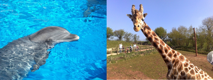
As an example, suppose you are interested in building a CNN to classify images as containing either dolphins or giraffes. To do this, let’s use an example data set that contains 94 images of dolphins and giraffes (Figure 2). To reproduce this example, you can download this data set from the SAS® Studio support website and unzip the contents to a location that is accessible to SAS Studio and to a SAS® Cloud Analytic Services (CAS) server.
Figure 2 Sample Images
After you extract the files, you can see that the dolphin and giraffe images are grouped into separate folders within the main giraffe_dolphin_small parent directory (Figure 3).
Figure 3 Image File Organization
This is a common way to organize images for classification so that the class labels can be automatically created by using the folder names when you load the images into SAS Studio.
Load and Display Your Images
The following code handles initial setup, loads the images into a data table in SAS, and displays a subset of them. To use the code, define the imagePath macro variable as the location where you unzipped the example data set.
/*** Macro variable setup ***/ /* Specify file path to your images (such as the giraffe_dolphin_small example data) */ %let imagePath = /filePathToImages/giraffe_dolphin_small/; /* Specify the caslib and table name for your image data table */ %let imageCaslibName = casuser; %let imageTableName = images; /* Specify the caslib and table name for the augmented training image data table */ %let imageTrainingCaslibName = &imageCaslibName; %let imageTrainingTableName = &imageTableName.Augmented; /*** CAS setup ***/ /* Connect to a CAS server */ cas; /* Automatically assign librefs */ caslib _all_ assign; /*** Load and display images ***/ /* Create temporary caslib and libref for loading images */ caslib loadImagesTempCaslib datasource=(srctype="path") path="&imagePath" subdirs notactive;libname _loadtmp cas caslib="loadImagesTempCaslib"; libname _tmpcas_ cas caslib="CASUSER"; /* Load images */ proc cas; session %sysfunc(getlsessref(_loadtmp)); action image.loadImages result=casOutInfo / caslib="loadImagesTempCaslib" recurse=TRUE labelLevels=-1 casOut={caslib="&imageCaslibName", name="&imageTableName", replace=TRUE}; /* Randomly select images to display */ nRows=max(casOutInfo.OutputCasTables[1, "Rows"], 1); _sampPct_=min(5/nRows*100, 100); action sampling.srs / table={caslib="&imageCaslibName", name="&imageTableName"}, sampPct=_sampPct_, display={excludeAll=TRUE}, output={casOut={caslib="CASUSER", name="_tempDisplayTable_", replace=TRUE}, copyVars={"_path_" , "_label_" , "_id_"}}; run; quit; /* Display images */ data _tmpcas_._tempDisplayTable_; set _tmpcas_._tempDisplayTable_ end=eof; _labelID_=cat(_label_, ' (_id_=', _id_, ')'); if _n_=1 then do; dcl odsout obj(); obj.layout_gridded(columns: 4); end; obj.region(); obj.format_text(text: _labelID_, just: "c", style_attr: 'font_size=9pt'); obj.image(file: _path_, width: "128", height: "128"); if eof then do; obj.layout_end(); end; run; /* Remove temporary caslib and libref */ caslib loadImagesTempCaslib drop; libname _loadtmp; libname _tmpcas_;
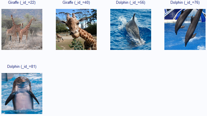
In addition to automatically extracting the class labels from the folder names, the code creates a unique ID variable (_id_) for each image. Both the label and the ID variable display above each image in the results by default (Figure 4).
Figure 4 Sample Images
The Load Images task enables you to easily customize how you load and display the images in SAS Studio. For more information, watch the companion video on YouTube and see the SAS Studio Task Reference Guide.
Explore and Process Your Images
Now that the images are in a data table in SAS, you can use the following code to explore the images by looking at summary information and label frequencies:
/*** Explore images ***/
proc cas;
    /* Summarize images */
    action image.summarizeImages /
                table={caslib="&imageCaslibName", name="&imageTableName"};

    /* Label frequencies */
    action simple.freq /
                table={caslib="&imageCaslibName", name="&imageTableName",
                       vars="_label_"};
    run;
quit;
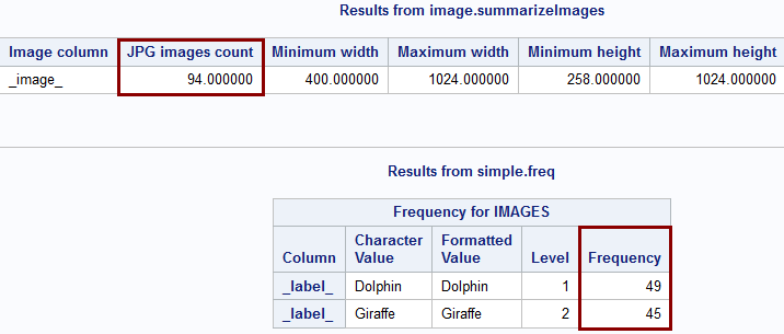
Figure 5 Summary Statistics
As expected, the data table contains 94 images (Figure 5), and for the class distribution, you can see that there are slightly more dolphins (49) than giraffes (45).
Next, let’s perform some common preprocessing steps for the images. First, you want to resize your images to match the image size that is required for one of the models you want to use. After resizing, you randomly shuffle the images. Initially, the dolphin and giraffe images are grouped together in the image table. This can cause problems when you train your model because it biases the parameters to overpredict a certain class. Shuffling alleviates this issue. Finally, you randomly partition your images into training and validation sets.
/*** Process images ***/
proc cas;
    /* Resize images to 224x224 */
    action image.processImages /
                table={caslib="&imageCaslibName", name="&imageTableName"}
                imageFunctions={{functionOptions={functionType='RESIZE',
                                                  height=224, width=224}}}
                casOut={caslib="&imageCaslibName", name="&imageTableName",
                        replace=TRUE};

    /* Shuffle images */
    action table.shuffle /
                table={caslib="&imageCaslibName", name="&imageTableName"}
                casOut={caslib="&imageCaslibName", name="&imageTableName",
                        replace=TRUE};

    /* Partition images */
    action sampling.srs /
                table={caslib="&imageCaslibName", name="&imageTableName"},
                sampPct=50,
                partInd=TRUE
                output={casOut={caslib="&imageCaslibName",
                                name="&imageTableName", replace=TRUE},
                        copyVars="ALL"};
    run;
quit;
Another common step in preprocessing images is data augmentation. You can augment the data in a number of ways, such as by cropping, rotating, or flipping your original images. This creates synthetic images to enlarge your training data, which is especially helpful when your training data set is small, as in our case.
The following code creates cropped versions of your images and then resizes them to match the rest of the images:
/*** Augment the training data ***/
proc cas;
    /* Create cropped images */
    action image.augmentImages /
                table={caslib="&imageCaslibName", name="&imageTableName",
                       where="_partind_=1"},
                cropList={{x=0,
                           y=0,
                           width=200,
                           height=200,
                           stepSize=24,
                           outputWidth=224,
                           outputHeight=224
                           sweepImage=TRUE}},
                casOut={caslib="&imageTrainingCaslibName",
                        name="&imageTrainingTableName", replace=TRUE};

    /* Label frequencies */
    action simple.freq /
                table={caslib="&imageTrainingCaslibName",
                       name="&imageTrainingTableName", vars="_label_"};
    run;
quit;
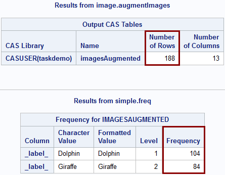
Figure 6 Data Augmentation Results
The original training partition contains 47 images, but the augmented training data contain 188 images (Figure 6).
Build and Train a Simple CNN Model
After you explore and prepare your data set, you can build and train CNNs to classify images. For the first model, let’s manually build the architecture from scratch.
You first create an empty deep learning model with the name and type that you specify. Let’s name it Simple_CNN and specify CNN as the model type. The model is stored as an in-memory table, and the name is how you subsequently use and interact with the model.
/*** Build model architecture ***/
proc cas;
    /* Create empty deep learning model */
    action deepLearn.buildModel /
               modelTable={name="Simple_CNN", replace=TRUE} type="CNN";
    run;
quit;
You then add layers to the model to slowly and flexibly define the network architecture. For each layer, you identify the model to add the layer to, in addition to specifying the name and type of the layer. You can also specify the hyperparameters specific to the layer type, such as the activation function (act) and number of filters (nFilters) for a convolutional layer. Typically, you also specify the source layers (srcLayers) that provide the inputs for the new layer.
For this simple model, let’s add two sets of convolutional and pooling layers, and then feed these into a fully connected layer before using a softmax output layer to generate the estimated probabilities for each class.
proc cas;
    /* Use the channel means as offsets */
    action image.summarizeImages result=summary /
                table={caslib="&imageTrainingCaslibName",
                       name="&imageTrainingTableName"};
    offsetsTraining=summary.Summary[1, {"mean1stChannel","mean2ndChannel",
                                        "mean3rdChannel"}];

    /* Add input layer */
    action deepLearn.addLayer /
                model="Simple_CNN"
                name="data"
                layer={type='input', nchannels=3, width=224, height=224,
                       offsets=offsetsTraining};
    /* Add convolutional layer */
    action deepLearn.addLayer /
                model="Simple_CNN"
                name="conv1"
                layer={type='convo', act="relu", nFilters=8, width=7, height=7,
                       stride=1}
                srcLayers={'data'};
    /* Add pooling layer */
    action deepLearn.addLayer /
                model="Simple_CNN"
                name="pool1"
                layer={type='pool', pool='max', width=2, height=2, stride=2}
                srcLayers={'conv1'};
    /* Add convolutional layer */
    action deepLearn.addLayer /
                model="Simple_CNN"
                name="conv2"
                layer={type='convo', act="relu", nFilters=8, width=7, height=7,
                       stride=1}
                srcLayers={'pool1'};
    /* Add pooling layer */
    action deepLearn.addLayer /
                model="Simple_CNN"
                name="pool2"
                layer={type='pool', pool='max', width=2, height=2, stride=2}
                srcLayers={'conv2'};
    /* Add fully connected (fc) layer */
    action deepLearn.addLayer /
                model="Simple_CNN"
                name="fc1"
                layer={type='fc', n=16, act='relu', init='xavier',
                       includeBias='true'}
                srcLayers={'pool2'};
    /* Add output layer */
    action deepLearn.addLayer /
                model="Simple_CNN"
                name="output"
                layer={type='output', n=2, act='softmax'}
                srcLayers={'fc1'};
    run;
quit;
After you build the architecture, you use the augmented training data set to train your model by using the deepLearn.dlTrain action, as follows:
/*** Train model with augmented training data ***/
proc cas;
    action deepLearn.dlTrain /
                table={caslib="&imageTrainingCaslibName",
					   name="&imageTrainingTableName"}
                model='Simple_CNN'
                modelWeights={name='Simple_CNN_weights',
                              replace=1}
                inputs='_image_'
                target='_label_' nominal='_label_'
                optimizer={minibatchsize=2,
                           algorithm={learningrate=0.0001},
                           maxepochs=10,
                           loglevel=2}
                seed=12345;
    run;
quit;
You can then use the trained model to score other images, and you can use a confusion matrix to assess the model’s performance.
/*** Score validation set with trained model ***/
proc cas;
    action deepLearn.dlScore /
                table={caslib="&imageCaslibName", name="&imageTableName",
                       where="_partind_=0"}
                model='Simple_CNN'
                initWeights={name='Simple_CNN_weights'}
                casout={caslib="&imageTrainingCaslibName",
                        name='imagesScoredSimpleCNN', replace=1}
                copyVars={'_label_', '_id_'};
    run;
quit;

/*** Create confusion matrix to assess performance ***/
proc cas;
   action simple.crossTab /
                row="_label_",
                col="_DL_PredName_",
                table={caslib="&imageTrainingCaslibName",
                       name='imagesScoredSimpleCNN'};
    run;
quit;
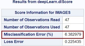
Figure 7 Simple CNN Model Validation Error
In the results (Figure 7), you can see that this simple CNN model performs fairly well, with a misclassification rate of only about 6% on the validation set. However, in general, building a model from scratch is very challenging, because to define the model architecture and to estimate the model you must specify many different hyperparameters. Also, training the model often takes a lot of time, computational resources, and training data for it to perform very well.
Instead of reinventing the wheel, an easier and more practical approach is to take a well-performing model that someone else already trained and apply it to your problem. This is known as transfer learning.
Transfer Learning with ResNet50
To demonstrate transfer learning, let’s use a popular CNN model known as ResNet50, which has been shown to perform very well for image classification, and let’s use your image data set to fine-tune the model for your application.
Just like before, you first need to define the model architecture as in the following code. This code uses an external .SAS file (model_resnet50_sgf.sas), because it takes about 700 lines of code to define the architecture for such a deep network. The code is a modified version of the model_resnet50.sas file available in the model utilities ZIP file from the SAS Deep Learning Models and Tools website. This website contains the SAS code and pretrained weights to build a few of the popular deep learning models, including ResNet50.
For this example, you need to download the ZIP file that contains the pretrained weights and other supporting files for the ResNet50 model. Place the contents of this file, along with the model architecture file (model_resnet50_sgf.sas), in a directory that is accessible to SAS Studio and to your CAS server. In the code, use the file path to the directory that contains the model files to define the modelPath macro variable.
/* Specify file path to the model files (.SAS architecture file, pretrained weights) */
%let modelPath = /filePathToModelFiles/;

/* Specify the name of the caslib associated with &modelPath */
%let modelCaslibName = dlmodels;

/*** Setup ***/
/* Create caslib with model files */
caslib &modelCaslibName datasource=(srctype="path") path="&modelPath"
    subdirs notactive;

/*** Build model architecture (using .sas file) ***/
proc cas;
    /* Include code to define ResNet50 architecture */
    ods exclude all;
    %include "&modelPath.model_resnet50_sgf.sas";
    ods exclude none;

    /* View model information */
    action deepLearn.modelInfo /
                modelTable={name="ResNet50"};
    run;
quit;
Next, use the following code to import the pretrained weights and associate them with your model:
/*** Import Caffe weights (in HDF5 format) ***/
proc cas;
    /* Import pretrained weights */
    action deepLearn.dlImportModelWeights /
                modelTable={name="ResNet50"}
                modelWeights={name='ResNet50_weights', replace=1}
                formatType="caffe"
                weightFileCaslib="&modelCaslibName"
                weightFilePath="ResNet-50-model.caffemodel.h5";
    run;
quit;
To set up this model, another thing to keep in mind is that ResNet50 was originally trained on the famous ImageNet data set, which contains 1,000 different classes. However, in this application, there are only two classes, so you need to remove the original output layer (fc1000) and replace it with an output layer that contains only two units (fc2).
/*** Change output layer to have the correct number of classes ***/
proc cas;
    /* Remove trained output layer */
    action deepLearn.removeLayer /
                modelTable={name="ResNet50"}
                name="fc1000";

    /* Add output layer with correct number of classes */
    action deepLearn.addLayer /
                model={name="ResNet50"}
                name="fc2"
                layer={type="output", n=2, act="softmax"}
                srcLayers={"pool5"};
    run;
quit;
Now that everything is set up, you can use your data to fine-tune ResNet50 for your application and then score the validation data. The following training code is essentially the same as the previous training code, except now you use the initWeights parameter to initialize the model weights by using the pretrained weights to fine-tune those weights with your data.
/***   Train model with augmented training data  ***/
/*** Initialize with pretrained ResNet50 weights ***/
proc cas;
    action deepLearn.dlTrain /
				table={caslib="&imageTrainingCaslibName",
                         name="&imageTrainingTableName"}
                model={name="ResNet50"}
                initWeights={name='ResNet50_weights'}
                modelWeights={name='ResNet50_weights_giraffe', replace=1}
                inputs='_image_'
                target='_label_' nominal={'_label_'}
                optimizer={minibatchsize=1,
                           algorithm={method='VANILLA', learningrate=5E-3}
                           maxepochs=5,
                           loglevel=3}
                seed=12345;
    run;
quit;

/*** Score validation set with trained model ***/
proc cas;
    action deepLearn.dlScore /
                table={caslib="&imageCaslibName", name="&imageTableName",
                       where="_partind_=0"}
                model={name="ResNet50"}
                initWeights={name='ResNet50_weights_giraffe'}
                casout={caslib="&imageTrainingCaslibName",
                        name='imagesScoredResNet50', replace=1}
                copyVars={'_label_', '_id_'};
    run;
quit;
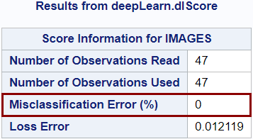
Figure 8 Fine-Tuned ResNet50 Model Validation Error
Keeping in mind that the validation set is not very large, the ResNet50 model can perfectly classify every image in the validation set (Figure 8), so it outperforms our simple CNN model.
The following video explains biases that can result from transfer learning (specifically frequency and context biases) and suggests ways to avoid them:
Put It to Work: Model Deployment
The final step is to save the information for this champion model as an analytic store.
/*** Create analytic store (astore) table to put model into production ***/
proc cas;
    action deepLearn.dlExportModel /
                modelTable={name="ResNet50"}
                initWeights={name="ResNet50_weights_giraffe"}
                casOut={name="ResNet50_giraffe"};
    run;
quit;
You can use this portable model format to easily deploy and manage the model by using SAS® Model Manager software or to make real-time decisions by using SAS® Event Stream Processing software.
As you can see, you can easily develop SAS code to cover the entire analytics life cycle—from data to discovery to deployment—to build a deep learning model for image classification. For more information about computer vision from SAS, check out Computer Vision: What It Is and Why It Matters.
Acknowledgments
The inspiration for this example comes from a SAS DLPy image classification example. DLPy is a high-level Python library for SAS Deep Learning. The author is grateful to Ed Huddleston at SAS Institute Inc. for his valuable editorial assistance in preparing this article. Thanks also to Anna Brown and Robert Blanchard for their helpful comments on an early draft.
References
Xian, Y., Lampert, C. H., Schiele, B., and Akata, Z. (2018). “Zero-Shot Learning—A Comprehensive Evaluation of the Good, the Bad and the Ugly.” IEEE Transactions on Pattern Analysis and Machine Intelligence (T-PAMI) 40:2251−2265 (arXiv:1707.00600 [cs.CV]).
Recommended Resources
In addition to the resources mentioned in the article, the following resources provide further information about deep learning from SAS:
- Mark as Read
- Mark as New
- Bookmark
- Permalink
- Report Inappropriate Content
Fantastic, that's a practical walk-through which can be easily re-created on your sas viya installation. the learning take-away is huge.
thanks
- Mark as Read
- Mark as New
- Bookmark
- Permalink
- Report Inappropriate Content
@acordes, thank you for the kind feedback, I'm really glad that the article was useful for you!
- Mark as Read
- Mark as New
- Bookmark
- Permalink
- Report Inappropriate Content
Great walk-through. One thing though, your last section says that the proc cas makes an astore file. I don't see how or where it creates an astore that can be used for deployment. It only creates a table in a session-scoped caslib that goes away when the session is over - thus, it is not deployable or portable as far as I can tell. Am I missing something and if so, can you explain more about the deployment piece? Deploying the model is arguably the most important part! To do that, I had to run "proc astore" to actually create the .astore file. Once I did that, I was able to bring the model into model manager (via import of the .astore).
- Mark as Read
- Mark as New
- Bookmark
- Permalink
- Report Inappropriate Content
@BrianGaines I want to know please if we can code Zero-Shot learning in SAS Guide? If not, can we do that in SAS Enterprise Miner or SAS Viya?
Catch up on SAS Innovate 2026
Nearly 200 sessions are now available on demand with the SAS Innovate Digital Pass.
Explore Now →SAS AI and Machine Learning Courses
The rapid growth of AI technologies is driving an AI skills gap and demand for AI talent. Ready to grow your AI literacy? SAS offers free ways to get started for beginners, business leaders, and analytics professionals of all skill levels. Your future self will thank you.

